Happiness…..I popped the pink pill into my mouth and waited for the expected feelings of ecstasy. No, the pill wasn’t the drug XTC, but rather a legal and safe “hacking” alternative. Then I put on my trans-cranial stimulation device, known as “The Thync,” and waited to see what happened. Wow! After five minutes, it felt like my brain was flooding me with endorphins. Finally, I placed the scalp stimulator known as the Tingler on my head. When I did this, an orgasmic wave of intense pleasure rippled through my entire body.
After a few minutes of this euphoria, I took off the devices and went about my day. Having just been catapulted into sweet ecstasy, my day became both incredibly productive and happy.
This is not a future scenario.
This is how I like to start my mornings. Nowadays, there are new and improved ways to feel good-even ecstatic-that most people don’t know anything about. In an age when depression is rampant and dangerous drug use is epidemic, amazing new ways to feel peaceful, euphoric, and just plain happy are popping up all over the place. However, people miss out on these amazing methods because they simply don’t know about them. From safe drugs to “happy apps,” to high tech brain stimulation devices, a whole new world of ways to feel good is blossoming.
We live in an age where everything is shifting and accelerating. Yet, most people still pursue an ancient path for finding happiness. Their formula for being happy is to try to control all the external events and people in their lives to be exactly the way they want. This is a tiresome activity at best, and there are always some events and people that we can’t control. However, there is a new model for finding more joy and peace of mind: find it within your self. Of course, this is a not a new idea. Everyone from the Buddha to Jesus has said that heaven can be found within, but now there are cutting edge and more efficient ways to tap into this magical inner kingdom.
As invited to talk to Google employees about “The Future of Happiness.” I described new ways to control their minds and emotions that were more effective than trying to be happy by controlling all the events in their life. The reaction was intense. Everyone wanted to know what some of these innovative ways to “hack happiness” were, and how they could get them. That led me to write a book on the subject.
In my research I learned that different things work for different people.
For example, there are a lot of supplements known as “cognitive enhancers” that can dramatically increase your focus, energy, and mood. Yet, you have to try out many of them in order to find the one or two that really rock your world. I also learned that people define happiness in unique ways. Some people want a gadget that increases their pleasure, while other folks want a tool that improves their relationships or makes them feel totally peaceful.
Gary Numan “Complex” from The Pleasure Principle
As with all technologies, “inner” tech keeps getting better. In fact, some of them are so good that it’s possible to get addicted to them. Ultimately, one has to discern whether a given gadget is truly a friend that helps them find the joy within–or is just another WMD-Widget of Mass Distraction. Since there are many tools that do different things, there’s no simple answer as to whether something is beneficial to you.
For example, people become addicted and dependent on coffee. Yet, on the other hand, caffeine can prevent many types of cancer, and helps people feel good and be productive. So, is coffee a “good” thing? It’s up to you to decide…
In my own case, I decide if a specific technology is truly my friend by asking myself two questions. First I ask myself, “Does this tool lead me to being dependent on it?” It’s always better when technology acts like “training wheels” on a bike-meaning that the tool exists so that you can eventually do without it. If instead a gadget fosters a sense of dependence, then that’s a warning sign it may ultimately not be worth it.
The second question is, “Does this technology help teach me how to better connect with a sense of peace, love, or joy within?” Even the Dalai Lama has reportedly said that if there were a pill that duplicated Buddha’s awakening, he would take it immediately and prescribe it for all living beings. If a tool helps me learn how to get to a more peaceful, loving place more efficiently, I think that’s a good thing.
It’s hard to say exactly what the future holds, though Steve Jobs was seemingly pretty good at predicting it. In 1972 I had the unusual opportunity to be in a computer class with Steve Jobs. Of course, at the time he was just a nerdy teen and I was four years his junior. He and I would vie to play Tic-tac-toe on a 500 pound “computer” that our High School had recently purchased. Steve was obsessed with this machine. One day I asked Steve why he was so fixated on this refrigerator sized computer. He turned to me and said in an intense manner, “Don’t you see? This machine is going to change everything! It’s going to change the world!”
It turns out Steve Jobs was right.
Well, nowadays it may not seem like the latest brain supplement, neuro-stimulator, or mood enhancing app is going to change the world, but technology has a way of discreetly slipping into our lives. This “technology of joy” will only accelerate until the entire way we pursue happiness is transformed in the next few years. I’ve seen that when people try out enough of these new gadgets, apps, and supplements, they inevitably find something that feels good–and is even good for them. When that happens, their lives are never the same. For the Silo,Jonathan Robinson.
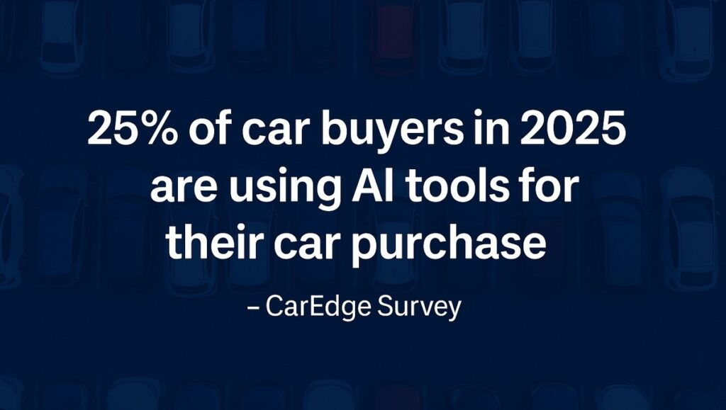
Amazon’s move into online car listings through Amazon Autos in 2024 has been widely framed as a breakthrough for consumers. But, for buyers considering this new option, the real story is more nuanced. While the platform offers a familiar, streamlined shopping experience and no-haggle pricing, it does not eliminate dealerships, negotiations behind the scenes, or the traditional profit structures that shape car pricing.
A quick heads up fellow Canucks- Amazon Autos is not yet available in Canada but plans are in place for expansion so stay tuned.
Trade Offs
As more North Americans explore buying a vehicle through alternative means including Amazon, experts say the key question isn’t whether it’s easier, but whether shoppers understand the trade-offs they’re making. Knowing the pros, the cons, and the fine print can be the difference between convenience and costly compromise.
What Works, What Doesn’t, and What to Watch For When Buying a Car on Amazon
Is It A True Breakthrough?
Amazon’s move into online car listings through Amazon Autos has been widely framed as a breakthrough for consumers. But, for buyers considering this new option, the real story is more nuanced. While the platform offers a familiar, streamlined shopping experience and no-haggle pricing, it does not eliminate dealerships, negotiations behind the scenes, or the traditional profit structures that shape car pricing. As more Americans explore buying a vehicle through Amazon, experts say the key question isn’t whether it’s easier, but whether shoppers understand the trade-offs they’re making. Knowing the pros, the cons, and the fine print can be the difference between convenience and costly compromise.
Amazon Autos, has generated headlines over the past year for a number of reasons. Some heralded the launch as a true game changer in the car market. But in reality, buying a car on Amazon is not all that different from buying a car the old fashioned way.
Participating automakers (like Hyundai) or dealers (like rental car giant Hertz) can now list their inventory on Amazon. But make no mistake: you’re still buying from a dealer. Amazon Autos is only acting as an online marketplace for cars, meaning that the cars you see listed are only there because traditional car dealers listed their inventory on the platform. Amazon is just making online car shopping feel like the Amazon experience that nearly 200 million Americans are familiar with.
There are pros and cons of buying a car on Amazon.
Amazon advertises no-haggle pricing, but there’s something crucial that most shoppers overlook: that rarely means you’re truly getting the best price possible. No-haggle pricing is crafted by dealers to ensure healthy profit margins on their end, while making consumers feel relieved that they don’t have to deal with unpleasant negotiations or salespeople. The truth is, buying the actual vehicle still takes place at a dealership. There are still salespeople involved. It can still be inconvenient or uncomfortable.
Dealers are thrilled with the assumption that pricing is already agreed upon before the customer even arrives. Remember, dealers have plenty of profit in the form of holdbacks, manufacturer-to-dealer cash, and even volume bonuses. That’s not to mention more money for them if you finance with them, or purchase an extended warranty or other add-on.
All of this means that you’re much more likely to overpay than if you were to go your own way and negotiate confidently.
In summary, when you buy a new or used car on Amazon, you’re still buying through a traditional dealership. Amazon doesn’t hold any of the inventory you see online, they’re merely adding the online Amazon experience many consumers are familiar with to online car shopping. In most cases, that means trading competitive pricing for convenience.
For some, that may be a compromise you’re willing to make in order to skip the haggling process. But it’s important to know that you’re limiting your ability to land a great deal when you forfeit your chance to negotiate car pricing.
Research Required
To best ensure you’re not leaving money on the table, thoroughly research the car market. Always research demand factors for the cars you’re interested in. Are you shopping for a car that’s less popular than the hottest sellers on the market? Does it sell slower than the market average in your area? If so, you’re much more likely to overpay with ‘no-haggle pricing’. Find inventory that has been sitting on the dealership lot the longest. Those are the cars that dealers are motivated to sell at a discount.
For the Silo, Justin Fischer.
Justin Fischer is an automotive retail analyst and consumer advocate at CarEdge, a leading consumer platform dedicated to empowering car shoppers to make confident, informed and financially savvy decisions.
Modern conveniences many take for granted — cell phones, laptops, GPS devices, even coffee makers — run on computer chips introduced by U.S. firms that established America’s leading role in technology. Trace the digital revolution, from its beginnings to the present day, with each groundbreaking advance.
How did these gains happen? Today’s technology emerged from U.S. support for research and development combined with America’s robust private sector, its scientific community, and its innovative spirit.
Bell Labs, a legendary research hub in New Jersey, began as a branch of the Western Electric Company, a subsidiary of the American Telephone and Telegraph Company (AT&T).
Founded in 1925 to meet a growing need for masscommunications, Bell Labs hired top engineers, physicists, chemists, and mathematicians to design and patent equipment (including a high-vacuum tube that transmitted telephone signals across North America).
Bell Labs encouraged interdisciplinary collaboration that produced groundbreaking discoveries. The labs were driven by scientific curiosity, flexible deadlines, and — thanks to AT&T’s budget — stable funding. Lab directors adopted a hands-off management style, and innovation flourished.
DID YOU KNOW?
In 1932, Bell Labs physicist Karl Jansky discovered radio waves coming from outer space. He’s known as the father of radio astronomy.
In the post-World War II period, Bell Labs’ Mervin Kelly assembled an all-star team of scientists to develop a replacement for the vacuum tube, which was bulky, fragile, and prone to burning out.
In 1947, John Bardeen and Walter Brattain — supervised by fellow physicist William Shockley — invented the point-contact transistor, a semiconductor device that amplifies sound and switches electrical currents on and off.
In 1948, Shockley designed the junction transistor, a more robust and reliable transistor. Its small size, low power consumption, and durability paved the way for computers, portable radios, cell phones, and other devices.
Eight years later, Bardeen, Brattain, and Shockley would be awarded the Nobel Prize in physics for this breakthrough.
DID YOU KNOW?
Bell Labs researchers have been awarded 10 Nobel Prizes in physics and chemistry, spanning from 1937 to 2023. While Bell Labs was at its most productive from the 1940s to the 1970s, important research continues today at its New Jersey headquarters.
Bell Labs continued to improve transistor technology during the 1950s, developing the silicon transistor and the metal-oxide-semiconductor field-effect transistor (MOSFET).
The MOSFET proved crucial for building high-density integrated circuits (ICs), or microchips, in the 1960s. Microchips — consisting of billions of tiny transistors crafted from semiconductor materials, commonly silicon — work together to power electronics.
Recognizing the potential for widespread impact and profits, Bell Labs created licensing agreements to share transistor technology with other companies.
In 1955, William Shockley left Bell Labs to establish Shockley Semiconductor Laboratory in Mountain View, California. Within a couple of years, some of his employees — engineers and scientists — formed their own company, Fairchild Semiconductor.
Fairchild is credited with the birth of Silicon Valley. The company became a major player in the growing semiconductor industry, and many Silicon Valley firms — including Intel (founded in 1968) and Apple (in 1976) — have ties to Fairchild alumni to this day.
As demand for semiconductors grew, so did the need for manufacturing capabilities.
Throughout the 1980s and 1990s, Japan, South Korea, and Taiwan became players in the industry, with Japanese companies like Toshiba and NEC influencing the data-storage market and South Korea’s Samsung and SK Hynix focusing on memory-chip production.
Meanwhile, the Taiwan Semiconductor Manufacturing Company (TSMC) upended a traditional business model of integrating chip design and manufacturing. It introduced the fabless-foundry model, encouraging firms to specialize in either design (fabless) or fabrication/manufacturing (foundry).
This increased efficiency. What’s more, it allowed many small firms — those lacking resources to open manufacturing plants — to design chips.
DID YOU KNOW?
The fabless-foundry business model democratized chip production, allowing startups to enter the market without the need for expensive manufacturing facilities.
Experts predict that quantum computing — with its ability to accelerate AI by overcoming limitations on data size, complexity, and processing speeds — will shape the future.
Quantum AI will develop algorithms that could advance pharmaceutical discoveries, predict financial outcomes, improve manufacturing, and bolster cybersecurity. Quantum/AI partnerships already comprise an active and developing market, with U.S. tech giants like IBM and Nvidia investing in both domains.
Industry leaders point to many factors that shape U.S. technological innovation. One such factor is the U.S. system of intellectual property protection, which fosters the spirit of risk-taking, says Walter Copan. (That system is enshrined in the U.S. Constitution, thanks to the foresight of America’s Founding Fathers.)
Sanjay Mehrotra cites the U.S. business culture of “openly, freely being able to debate ideas,” adding, “The best ideas win.”
Thomas Caulfield says, “This is where you can work hard, live your dream, become an entrepreneur, start a company.”
And Jon Gertner notes that key people at Bell Labs came from humble beginnings: “To me, that feels uniquely American — the idea that talent could rise from almost anywhere and shape the future of communications.”
It’s part of Silicon Valley lore that massive tech empires often sprouted from humble roots. As quantum computing and AI herald the next seismic shifts in technology, innovation hubs could emerge in unlikely places. Who knows? The next great U.S. tech companies might now be incubating in a town anywhere in America.
Ottawa’s forthcoming AI strategy needs to walk a tightrope between two equally important principles: safeguarding Canadians from possible misuses of AI but also giving our private and academic sectors the leeway to use Canada’s AI strengths to develop and commercialize new technologies and products.
Planned AI adoption rose sharply between Q3 2024 and Q3 2025, but progress remains highly uneven across industries. Knowledge-intensive sectors – such as information and cultural industries, finance and insurance, and healthcare – show the strongest gains, while several goods-producing and operational sectors, including manufacturing, wholesale trade, and mining, show stagnant or declining expectations.
The federal government must clearly define a framework for responsible, widespread AI innovation – one that encourages beneficial development and adoption while setting firm expectations about the harms innovators must avoid.
Canada’s competition reforms must keep pace with data-driven business models by empowering authorities with modern tools to detect, assess, and stop conduct that genuinely harms competition, innovation, or consumers.
The explosive growth of online shopping is reshaping Canadian retail by empowering consumers with unprecedented choice, driving omnichannel innovation, and intensifying competition.
MGO, a glucose metabolite, can temporarily destroy the BRCA2 protein, reducing its levels in cells and inhibiting its tumor-preventing ability.
Via friends at epochtimes. You may have heard that sugar feeds cancer cells, and evidence supports that. However, the missing link in this narrative has been a thorough understanding of just “how” sugar feeds cancer—until now. A study from 2024 published in Cell in April uncovered a new mechanism linking uncontrolled blood sugar and poor diet with cancer risk.
The research, performed at the National University of Singapore’s Cancer Science Institute of Singapore, and led by professor Ashok Venkitaraman and Li Ren Kong, a senior research fellow at the University of Singapore, found a chemical released when the body breaks down sugar also suppresses a gene expression that prevents the formation of tumors.
This discovery provides valuable insights into how one’s dietary habits can impact their risk of developing cancer and forges a clear path to understanding how to reverse that risk with food choices.
Methylglyoxal–A Temporary Off Switch
It was previously believed that cancer-preventing genes must be permanently deactivated before malignant tumors can form. However, this recent discovery suggests that a chemical, methylglyoxal (MGO), released whenever the body breaks down glucose, can temporarily switch off cancer-protecting mechanisms.
Mr. Kong, first author of the study, stated in a recent email: “It has been shown that diabetic and obese individuals have a higher risk of cancer, posing as a significant societal risk. Yet, the exact cause remains debatable.
“Our study now unearthed a clue that may explain the connection between cancer risk and diet, as well as common diseases like diabetes, which arise from poor diets.
“We found that an endogenously synthesized metabolite can cause faults in our DNA that are early warning signs of cancer development, by inhibiting a cancer-preventing gene (known as the BRCA2).”
BRCA2 is a gene that repairs DNA and helps make a protein that suppresses tumor growth and cancer cell proliferation. A BRCA2 gene mutation is associated primarily with a higher risk of developing breast and ovarian cancers, as well as other cancers. Those with a faulty copy of the BRCA2 gene are particularly susceptible to DNA damage from MGO.
However, the study showed that those without a predisposition to cancer also face an increased risk of developing the disease from elevated MGO levels. The study found that chronically elevated levels of blood sugar can result in a compounded increase in cancer risk.
“This study showcases the impact of methylglyoxal in inhibiting the function of tumour suppressor, such as BRCA2, suggesting that repeated episodes of poor diet or uncontrolled diabetes can ‘add up’ over time to increase cancer risk,” Mr. Kong wrote.
The Methylglyoxal and Cancer Relationship
MGO is a metabolite of glucose—a byproduct made when our cells break down sugar, mainly glucose and fructose, to create energy. MGO is capable of temporarily destroying the BRCA2 protein, leading to lower levels of the protein in the cells and thus inhibiting its ability to prevent tumor formation. The more sugar your body needs to break down, the higher the levels of this chemical, and the higher your risk of developing malignant tumors.
“Accumulation of methylglyoxal is found in cancer cells undergoing active metabolism,“ Mr. Kong said. ”People whose diet is poor may also experience higher than normal levels of methylglyoxal. The connection we unearthed may help to explain why diabetes, obesity, or poor diet can heighten cancer risk.”
MGO is challenging to measure on its own. Early detection of elevated levels is possible with a routine HbA1C blood test that measures your average blood sugar levels over the past two to three months and is typically used to diagnose diabetes. This new research may provide a mechanism for detecting early warning signs of developing cancer.
“In patients with prediabetes/diabetes, high methylglyoxal levels can usually be controlled with diet, exercise and/or medicines. We are aiming to propose the same for families with high risk of cancers, such as those with BRCA2 mutation,” Mr. Kong said.
More research is needed, but the study’s findings may open the door to new methods of mitigating cancer risk.
“It is important to take note that our work was carried out in cellular models, not in patients, so it would be premature to give specific advice to reduce risk on this basis. However, the new knowledge from our study could influence the directions of future research in this area, and eventually have implications for cancer prevention,” he said.
“For instance, poor diets rich in sugar or refined carbohydrates are known to cause blood glucose levels to spike. We are now looking at larger cancer cohorts to connect these dots.”
The Diet and Cancer Connection
Dr. Graham Simpson, medical director of Opt Health, stated in an email: “It’s genes loading the gun, but your lifestyle that pulls the trigger. Every bite of food you take is really information. It’s either going to turn on your longevity genes or it’s going to turn on your killer genes. So cancer is very much in large part self-induced by the individual diet.”
A 2018 study published by Cambridge University Press found an association between higher intakes of sugar-sweetened soft drinks and an increased risk of obesity-related cancers. Research published in the American Journal of Clinical Nutrition in 2020 concluded that sugars may be a risk factor for cancer, breast cancer in particular. Cancer cells are ravenous for sugar, consuming it at a rate 200 times that of normal cells.
Healthy Dietary Choices for Reducing Cancer Risk
A consensus on the best dietary approach for reducing cancer risk has yet to be determined, and further research is needed. However, the new findings of the Cell study on MGO support reducing sugar intake as a means to mitigate cancer risk. A study published in January in Diabetes & Metabolism shows that a Mediterranean diet style of eating may help reduce MGO levels.
In 2023, a study published in Cell determined that a ketogenic diet may be an effective nutritional intervention for cancer patients as it helped slow the growth of cancer cells in mice—while a review published in JAMA Oncology in 2022 found that the current evidence available supports a plant-enriched diet for reducing cancer risk.
Dr. Simpson stressed the importance of real food and healthy macronutrients with a low-carb intake for the health of our cells. “The mitochondria is the most important signaling molecule and energy-producing organelle that we have in our body. [Eat] lots of vegetables, healthy proteins, and healthy fats, fish, eggs, yogurt,” he said.
“Lots of green, above-ground vegetables, some fruits, everything that is naturally grown and is not processed.” For the Silo, Jennifer Sweenie.
Inaugural U.S.-Africa Technical and Regulatory Space Training Meeting
December, 2025. Senior Bureau Official (SBO) in the Bureau of African Affairs Ambassador Jonathan Pratt convened today’s U.S.-Africa Technical and Regulatory Space Training Meeting, the first in a series of technical and regulatory trainings in the leadup to the NewSpace Africa Conference April 20-23, 2026 in Libreville, Gabon.
SBO Pratt conveyed that the United States aims to empower African nations to create locally owned, financially sound, and internationally-aligned space programs – not dependent, opaque, or controlled by outside actors.
This meeting represented the first step in the United States deepening space diplomacy on the African continent, now with more than 60 satellites in orbit. Representatives agreed to work more closely together to advance responsible exploration in space and collaborate transparently and openly.
Participating in the meeting were representatives from the following African space agencies: Senegal, Angola, Mauritius, Djibouti, Nigeria, Kenya, Botswana, Gabon, Ethiopia, Namibia, Rwanda, and Egypt. The meeting also included representatives from the Department of War, Department of Commerce, and the Federal Communications Commission.
Supplemental
With a total of 13 satellites each, South Africa and Egypt have the largest number of satellites in orbit in Africa, while Nigeria also launched a total of seven satellites, according to a report by Statista.
Take a look at the list of African countries with the most satellites in orbit as of August 2024:
country
number of satellites
South Africa
13
Egypt
13
Nigeria
7
Algeria
6
Morocco
3
Since the statistics were published, Morocco launched two more nanosatellites, bringing the total number of satellites to five.
The report also noted that 12 other African countries had satellites in space, namely Kenya, Angola, Ethiopia, Rwanda, Djibouti, Ghana, Mauritius, Senegal, Tunisia, Sudan, Uganda, and Zimbabwe.
South Africa was the first country on the continent to build and launch a satellite, called SUNSAT-1, in 1998.
The first outing of the European lunar rover MONA LUNA reflects the collective work of Venturi Space’s three sites. Monaco, Switzerland and France worked hand‑in‑hand to design, develop, assemble and test the rover.
Weighing 750 kg (extendable to 1,000 kg), MONA LUNA will serve two primary objectives: to explore the lunar surface and to test critical technologies for sustainable lunar mobility. Thanks to its four wheel‑drive and four‑wheel steering system, along with passive‑damping suspension, MONA LUNA climbed and descended slopes of up to 33 degrees, exceeding initial expectations. The first results confirm the rover’s potential: The contact area of the hyper‑deformable wheels is exceptional, both on loose soil and rolling terrain.
This confirms the findings of intensive tests carried out at NASA between 2022 and 2025,Traction exceeds forecasts, Large rocky obstacles are crossed effortlessly, Dynamic stability on slopes meets programme requirements, The onboard electronic systems demonstrated excellent operational performance. Designed to support the ambitions of the European Space Agency (ESA) and France’s Centre National d’Études Spatiales (CNES), MONA LUNA already incorporates technologies that will operate on the Moon next summer — but on board another rover: FLIP. This vehicle will be equipped with the same hyper‑deformable wheels, batteries, heating systems and temperature sensors as the European rover. FLIP is developed by the North American company Venturi Astrolab, Venturi Space’s strategic partner. FLIP will also benefit from another innovative technology developed by Venturi Space: the mechanical system enabling the rover to exit the lunar lander.
Another shared feature between MONA LUNA and FLIP is their bodywork, designed by Sacha Lakic.In parallel with the MONA LUNA development programme, Venturi Space continues to expand its industrial ecosystem and will lay the first stone of its flagship facility next spring: a site of more than 10,000 m² in Toulouse, just steps away from the Centre National d’Études Spatiales (CNES). It is here that, in the first half of 2028, 150 engineers will work on the design and manufacturing of MONA LUNA, in close collaboration with the Swiss and Monegasque entities responsible for the hyper‑deformable wheels, heating systems, cryogenic materials, the rover‑lander egress system, and the high‑performance batteries.
Quotes Daniel Neuenschwander, Director of Human and Robotic Exploration at the ESA: “I was truly impressed by the way MONA LUNA handled LUNA’s challenging terrain. Watching its wheels deform and adapt to the regolith, slopes and rocks… it is remarkable. If MONA LUNA were to be selected for one of our missions, it would be a tremendous opportunity for Europe.”
Gildo Pastor, President of Venturi Space: “Seeing MONA LUNA operate on the legendary LUNA site is a profound source of pride. This rover demonstrates the performance of our wheels, our suspension systems, our electronics… and therefore the quality of the work achieved by all our teams in Toulouse, Monaco and Switzerland. We know we have only completed 1% of the journey that, I hope, will take us to the Moon.”
Dr. Antonio Delfino, Director of Space Affairs at Venturi Space: “These driving tests were primarily dedicated to locomotion. We wanted to understand how MONA LUNA behaves on loose soil, on slopes and when facing significant obstacles. The results exceed our expectations. The ability of these wheels to ‘float’ on the surface is essential to avoid becoming bogged down in lunar regolith.”
The tiny home sector is big on innovation as exemplified by a new crop of amazing Accessory Dwelling Unit (ADU) designs across the U.S. and Canada showcasing state-of-the-art architectural and interior features, thoughtful layouts and stunning aesthetics that redefine what’s possible in small-space living. Maxable—North America’s leading provider of resources for building guest houses, casitas, in-law suites, granny flats, pool houses and other ADUs—has officially named the the #1 best ADU of 2025 and other of the ’10 Best’ for the year based on a mix of criteria: visual appeal, use of space, creativity and functionality. Multiple photos for each are showcased online demonstrating the extreme ingenuity of each build.
Every year, Maxable’s ‘Best ADU of the Year’ competition celebrates the most innovative and impressive tiny home projects from across North America. Accessory dwelling units (ADUs) that don’t just look great, but solve real challenges of space, budget, and lifestyle. And the Top 10 have just been named! “If there’s one thing we’ve learned this year, it’s that accessory dwelling units ADUs aren’t going anywhere,” says Maxable CEO Paul Dashevsky. “In fact, they’re chugging along at full force as new regulations make their mark, homeowners are letting their creativity bloom, and designers are pushing the limits of what’s possible in small-space living.”
Here is the #1 winner and other of the top 10 best ADUs that have earned their keys in 2025. ______________________________________________________
#1 Best ADU of 2025:
Ashby ADU, Piedmont, CA
Designer: Tuan Le Design
Builder: Atelier19AD6
Size: 800 sq ft, 2 bed, 1 bath
Built on a steep slope, the project faced challenges with utility coordination, subcontractors, supply chain delays, and neighbor considerations, yet the team navigated every obstacle to deliver a standout result. The unit is fully electric, with a heat pump, water heater, and solar panels, making it efficient and environmentally conscious. Skylights and floor-to-ceiling four-panel sliding glass doors fill the interior with natural light, creating a bright, airy atmosphere. The modern design continues on the exterior with sleek wood paneling that complements the contemporary interior. The result is a stylish, functional ADU that maximizes both the views and the livable space
Other Top 10 Best ADUs of 2025
Chamomile Cottage, Arlington, MA
Modular Design and Build: Backyard ADUs
Size: 567 sq ft, 1 bed, 1 bath
If a cozy cup of tea was an ADU, we think it’d look like this! Designed to bring an aging father closer to his family and young grandchildren, this modular build balances warmth, accessibility, and beautiful design. As one of the first detached ADUs completed under Massachusetts’ new ADU law, it also marks a milestone for backyard living in the state. Built with collaboration between Backyard ADUs and a homeowner with impeccable design taste, the result is both functional and heartfelt. Chevron wood flooring, warm olive walls, and a charming fireplace make the space feel like home from the moment you step inside. Skylights fill the rooms with natural light, while the ADA-compliant bathroom ensures comfort and safety for years to come.
Alora ADU, San Diego, CA
Designer: Ruland Design Group
Builder: Glann Fick, Coastline Construction
Size: 1,000 sq ft, 2 bed, 2 bath duplex
This project is a beautiful example of how ADUs can bring generations together while adding long-term value to a property. The homeowners created not one, but two attached backyard homes. One was designed for an aging mother, and the other for rental income to support the family. Together, the units make space for four generations to stay close while still maintaining privacy and independence. Both ADUs were designed with light, openness, and connection to the outdoors in mind. High ceilings and clerestory windows fill the interiors with natural light, while large sliding glass doors open to private patios for easy indoor-outdoor living. Each space feels modern and welcoming, complete with well-appointed kitchens and roomy islands perfect for family meals or morning coffee. It’s a true example of multigenerational living done right.
Copperline ADU, San Diego, CA
Designer and Builder: SnapADU
Size: 980 sq ft, 2 bed, 2 bath
This Spanish-style ADU in Rancho Santa Fe was designed to blend seamlessly with the community’s strict architectural standards. The homeowner, a roofing contractor, personally installed the boosted tile roof to match the main home, turning HOA requirements into an opportunity to create a timeless retreat. Today, the ADU serves as a private space for family and guests. Every element, from hand-textured stucco to arched porch openings and copper gutters, was carefully chosen to mirror the primary residence. Inside, faux wood ceiling beams add warmth to the great room, while custom shelving and professional-grade appliances enhance the kitchen. Each bedroom features an ensuite bath and walk-in closet, with a back entrance leading to a mudroom and laundry area.
Brick House ADU, Denver, CO
Designer and Builder: ADU4U
Size: 938 sq ft, 1 bed, 1.5 bath
This ADU project breathes new life into an old, historic building, while preserving its authentic character and respecting its roots. Building a modern structure within an 138 year old structure was an innovative solution to achieve this. In historic Curtis Park, Denver’s oldest neighborhood, an 1886 brick carriage house stands as a testament to the passage of time. The building sits inside the boundaries of Denver’s historic Curtis Park, so all exterior design and material selections had to be approved through the city’s Landmark Commission.
ADU4U turned this once-unlivable structure into a cozy, modern home while preserving its historic charm. To bring it up to today’s safety standards, the team strengthened the old brick with a new steel frame and carefully reused original materials throughout the interior. The hayloft door became the powder room door, and the old floor joists were turned into a beautiful kitchen peninsula. Now, this light-filled ADU perfectly balances historic character with modern comfort. It’s truly a shining example of how old buildings can be reimagined for today’s living.
Longview ADU, Washington D.C.
Designer: Ileana Schinder
Builder: J Cabido Designs
This project is a creative transformation of an abandoned garage and storage space into a bright and efficient one-bedroom ADU. By keeping the original structure’s footprint, the design team minimized both construction costs and the visual impact on the surrounding property. Every detail was planned with sustainability in mind. From upgraded insulation to energy-efficient mini splits and an energy recovery ventilator, the ADU meets Washington DC’s strict environmental standards while maintaining year-round comfort. Restoring the building’s existing openings allowed natural light to flood the interior, creating a warm and inviting space that feels much larger than its footprint. The result is a thoughtful blend of preservation, sustainability, and smart design, breathing new life into what was once an overlooked structure.
Sagebrush ADU, Menlo Park, CA
Designer: Inspired ADUs
Builder: Integrum Construction
This ADU is a masterclass in craftsmanship and timeless design. Every detail, from the cedar shake siding to the copper flashings, was carefully chosen to mirror the main home and create a seamless, cohesive look. Instead of competing with the original architecture, it enhances it, feeling like it has always been part of the property. Natural materials play a starring role here. The cedar and copper will continue to age beautifully, adding warmth and character over time. Inside, handmade tile, custom cabinetry, and a cozy loft make the space feel elevated yet inviting. Every inch was designed with intention, balancing function, beauty, and authenticity. This ADU proves that small-scale construction can be both refined and enduring.
Brushstroke ADU, Newcastle, CA
Designer and Builder: A+ Construction ADU Builders
Size: 1,198 sq ft + 800 sq ft deck, 3 bed, 2 baths
The client didn’t want to separate three generations of their family, so they built a second home in their backyard. This ADU allows their parents to live independently with their own routines and art studio, while staying just steps from family dinners, grandkid hugs, and everyday life together. At 1,200 sq. ft., the ADU includes three bedrooms, two bathrooms, and a large open living area. The layout prioritizes comfort, easy movement, and aging-in-place, with wide circulation paths, direct deck access from the primary bedroom, and plenty of natural light. A dedicated art studio with custom cabinetry and large windows supports the grandmother’s creative routine. The best feature? An 800 sq. ft. covered deck and carefully chosen exterior finishes. All of these details make the ADU feel integrated with the main home, creating a thoughtful, functional, and long-term living space for the whole family.
Alcove ADU, Los Angeles, CA
Designer: Homeowner
Builder: Doobek Brothers
Size: 593 sq ft, 1 bed, 1 bath
What started as a retrofit for a carport turned into a fully functional ADU, making smart use of limited space while navigating strict city codes. Because the property sits on a hillside, any addition beyond the existing roofline would have required expensive drainage to the street, so the design works entirely within the original footprint. The interior feels calm and spacious thanks to thoughtful layout, finishes, and furniture. A double wall between the kitchen and bathroom cleverly hides appliances while providing storage for cleaning supplies, making the space feel open and uncluttered. Temperature and sound insulation reduce energy costs for both units, making it highly efficient. Windows were sized to align with the upstairs unit, creating visual harmony. With parking right outside and a potential deck planned for the upper unit, this ADU demonstrates how careful design can turn code restrictions into a livable home.
Elevare ADU, San Diego, CA
Designer: Sergio Perlata
Builder: HM Construction
Size: 479 sq ft, 1 bed, 1 bath
This daring ADU was built on top of the homeowner’s existing house to preserve the garage while creating a luxurious, functional space. What started as a bold idea and labor of love resulted in a retreat that balances comfort, style, and modern California living. The design maximizes natural light, features high-end finishes, and offers seamless indoor-outdoor flow. Privacy for the main house was carefully considered, and practical choices like spa-like micro-cement in the bathroom create a durable, low-maintenance, and rental-friendly space. More than just a guest house, this ADU is a thoughtfully crafted space that inspires relaxation and connection.
November, 2025 – The federal Canadian government is expected to unveil proposed changes to its electric vehicle sales mandate this winter. The upcoming announcement comes as Canada’s 2026 Zero Emissions Vehicle (ZEV) mandate – requiring 20 percent of new light-vehicle sales to be electric – faces mounting evidence it was unlikely ever to be met, according to a new report by the C.D. Howe Institute.
In “Mandating the Impossible? Assessing Canada’s Electric Vehicle Mandate for 2026 and Beyond,” Brian Livingston, at the C.D. Howe Institute, finds that the policy’s trajectory remains unrealistic beyond 2026. “Even if incentives return, the targets far exceed what consumers are willing or able to buy,” says Livingston. “Mandates alone won’t generate the demand or the vehicles needed to meet these goals.”
The analysis shows that under the 2026 requirement, automakers collectively would have had to spend hundreds of millions of dollars to comply. Companies falling short of their targets could face over $200 million in penalties to generate “Charging Fund Credits,” along with unknown additional costs to purchase “Excess Credits” from firms such as Tesla and Hyundai. To meet compliance thresholds, manufacturers might have been forced to restrict non-ZEV sales, reducing total vehicle supply by more than 400,000 units – leaving significant consumer demand unmet.
Meanwhile, companies exceeding the 20 percent target – primarily foreign-based automakers – would benefit from windfall revenues by selling excess credits. Canadian-based producers such as GM, Ford, Toyota, Stellantis, and Honda, which manufacture domestically, would bear higher costs and face reduced competitiveness.
Federal officials recently noted that the government’s highly anticipated review of the ZEV mandate – launched after Prime Minister Mark Carney paused the 2026 target in September – will report back this winter and unveil proposed changes to targets and credit rules.
Livingston recommends that Ottawa either abandon or substantially revise the ZEV mandate. Options include revising percentage targets to align with market realities, counting increasingly popular hybrid vehicles toward compliance, redirecting credit proceeds to the federal government, or suspending the mandate until trade negotiations with the United States and China clarify the future of Canada’s auto sector.
“The waiver of the 2026 target is only a first step,” Livingston cautions. “Unless the policy is recalibrated to reflect consumer demand and production capacity, Canada’s ZEV mandate risks driving up costs, shrinking supply, and undermining competitiveness – without delivering meaningful emissions reductions.”
AI is fundamentally redefining leadership by providing new tools, frameworks, and systems that allow leaders not just to manage complexity, but to see, challenge, and reshape their organizations in ways never before possible. The competitive mandate for leaders is clear: harness AI not merely for efficiency, but as an engine for deeper self-awareness, structured dissent, and proactive sensing that unlocks true organizational agility and resilience.
Strategic Frameworks for Next-Gen AI Leadership
Forward-thinking leaders are moving beyond pilot projects and isolated automation to experiment with new, holistic approaches—many inspired by concepts like the Leadership Mirror, Red-Team Loop, and Organization Pulse Monitor. These paradigms operationalize AI in ways that directly address the perennial blind spots, biases, and inertia that often undermine executive decision-making.
George Yang- helping organizations and executives embrace AI.
The Leadership Mirror: Cultivating Radical Self-Awareness
The Leadership Mirror uses AI to continuously analyze leadership communication, decision rationale, and team interactions, surfacing insights that are often overlooked or difficult for humans to acknowledge. For example, Microsoft has begun leveraging AI tools to track who dominates meetings, which voices get systematically dismissed, and when evidence is overridden by intuition—creating dashboards that encourage leaders to confront uncomfortable patterns.
This approach helps leaders challenge their own narrative, improve inclusiveness, and drive more thoughtful debate.
With AI’s ability to process language in real time, leaders can receive feedback loops and “reflections” that support a culture of deliberate, transparent leadership.
The Leadership Mirror is also a vehicle for mitigating the “competence penalty,” where women and older workers face skepticism for using AI—even when it enhances productivity. By surfacing evidence of expertise and impact, it reduces bias and builds psychological safety.
There are different types of AI including less sophisticated models such as Generative AI. To decide whether to use generative artificial intelligence for a task, ask yourself whether it matters if the output is true and you have the expertise to verify the tool’s output. (Adapted from Aleksandr Tiulkanov‘s LinkedIn post)
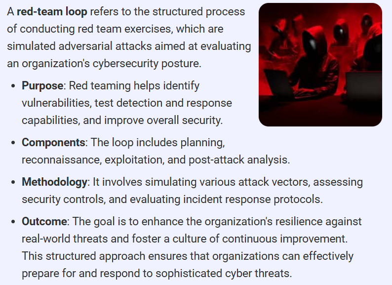
The Red-Team Loop: Embedding Structured Dissent
To counter groupthink and executive overconfidence, Red-Team Loop systems employ AI to automate adversarial reviews of strategy and operational decisions. Verizon, for instance, uses an AI framework that captures assumptions, risks, and anticipated outcomes for major decisions, then generates simulated critiques and alternative scenarios—sometimes challenging senior executives on blind spots they themselves hadn’t recognized.
By proactively “red-teaming” their own decisions, leaders foster a culture where dissent is routine, rational, and data-driven—not ad hoc or punitive.
The approach is especially valuable in M&A, crisis management, and product launches, where high-stakes, high-ambiguity decisions benefit from rigorous challenge.
Leading boards now expect Red-Team Loops as part of their fiduciary duty, recognizing that the cost of missed risks is measured not just in dollars, but reputation and long-term viability.
Organization Pulse Monitor: Proactive Sensing for Culture and Risk
The Organization Pulse Monitor uses AI to detect weak signals in organization culture, ethical risk, and operational friction long before traditional metrics or surveys would register them. Some organizations have begun linking AI-powered sentiment analysis of internal communications, workflow behaviors, and network interactions to predict where a culture may be straining, where compliance risks are emerging, or where silent dissent is brewing.
When Pulse Monitors flagged drops in engagement and early warning signs of burnout, one multinational fast-tracked well-being interventions, pre-empting attrition.
AI-driven pulse scans also help surface ethical risks—such as exclusionary behaviors or data privacy concerns—enabling leaders to respond immediately, not months later.
Actionable Strategies: Bringing AI Experiments to Leadership
How can senior leaders experiment and innovate with these systems while maximizing value and minimizing risk?
Map Adoption Hotspots and Blind Spots: Use mirror and pulse data to identify where AI is catalyzing positive behaviors—and where competence penalties or shadow AI usage may be undermining equity or performance. Target interventions accordingly.
Mobilize Role Model Leaders: Encourage respected senior leaders, particularly those from underrepresented demographics, to visibly experiment with and champion AI tools. Research shows that when these role models use AI openly, adoption gaps shrink, and psychological safety rises.
Redesign Evaluation and Disclosure Policies: Shift performance metrics from subjective ratings of proficiency to objective impact, cycle time, accuracy, and innovation. Blind reviews and private feedback mechanisms can reduce bias against AI users and drive fairer rewards.
Embed Structured Red-Teaming in Decision Flows: Institutionalize adversarial testing of key decisions, making AI-enabled dissent a standard step—not a threat or afterthought. Leaders should receive regular “contrarian” insights, not just consensus-building reports.
Common Pitfalls and Human Impact
Despite rising investment, less than one-third of US employers believe staff are equipped for critical thinking in the AI era, and only 16% of American workers use AI on the job despite widespread availability. The main barriers are not just technical, but social: competence penalties, fear of reputation loss, and resistance among influential skeptics.
Competence Penalty: AI users, especially women and older employees, may face a perception of diminished competence. This undermines adoption and can exacerbate workplace inequality.
Shadow AI and Hidden Risks: Employees sometimes use unauthorized tools to bypass bias, exposing the organization to compliance, reputational, and security risk.
Skill Gaps vs. Work Context: Traditional training falls short without tailored, role-specific feedback loops—AI tutors offer scalable, personal learning but must be embedded in daily workflow, not delivered in isolation.
Governance, Ethics, and Sustainable Change
Human-centered leadership isn’t optional—it’s a strategic imperative. Boards and executives must be proactive in:
Instituting transparent governance for all AI systems (mirrors, loops, monitors), with clear oversight on privacy, fairness, and impact.
Ensuring structured role-modeling and psychological safety—particularly for vulnerable groups confronting competence penalties.
Making change management a continuous process, with AI as both coach and sentinel, not just a dashboard.
The call to action for C-suite leaders is urgent and profound: treat responsible, experimental, and self-critical AI adoption as the core discipline of next-generation leadership. Not just for efficiency, but for building organizations where insight, challenge, and well-being are sustainably enabled. Those who master the trifecta of mirror, loop, and pulse will set the new standard for profitable, human-centered growth in the age of AI.
More about:
George Yang is a Toronto-based digital innovator and AI adoption strategist with over 15 years of experience in marketing and digital transformation. As Chair of the AI Working Group at the National Payroll Institute, he helps organizations translate AI strategy into measurable business outcomes. George is passionate about making AI adoption ethical, practical, and impactful, bridging the gap between innovation and implementation across industries. georgeyang.ca
From electro-chromatic e-windows to using supernova explosions to explore the earth for mineral deposits: World Economic Forum 2025 Technology Pioneers Leading New Wave of Global Innovation
The World Economic Forum selects 100 start-ups from 28 countries to join its Technology Pioneers community.
The new cohort marks a global surge of emerging technologies, from smart robotics and spatial AI to flying taxis and scalable quantum solutions.
Now in its 25th year, the community has recognized over 1,200 start-ups that have gone on to transform industries and societies worldwide.
For more information on the Annual Meeting of the New Champions 2025, visit wef.ch/amnc25 and share on social media using the hashtag #amnc25, or #2025夏季达沃斯#. Read more about the 2025 Technology Pioneers here.
Geneva, Switzerland, 2025 – The World Economic Forum 2025 Technology Pioneers community is a group of 100 early-stage companies from 28 countries driving innovation across industries and borders. Now in its 25th year, the program celebrates its strongest cohort yet, marked by broader geographical representation, greater diversity beyond Silicon Valley and the rise of more ambitious frontier technologies.
Reflecting wider shifts in the innovation landscape, many of the companies spotlighted are using artificial intelligence (AI) to reach greater scale and sophistication with fewer resources. Several are venturing into less explored frontiers – from asteroid mining and flying electric taxis, to leveraging satellite imagery to transform agriculture and harnessing energy from supernova explosions to locate critical minerals beneath the Earth’s surface.
The geography of innovation is also evolving.
While the United States remains the top contributor to the community, Europe’s share has surged to 28% – up from 20% last year – reflecting the rise of strong tech ecosystems across the region. China and India are also emerging as major tech innovation hubs.
“There has never been a more exciting time to dive headfirst into tech innovation. But no one gets far alone – you need a community to move your mission forward,” said Verena Kuhn, Head of Innovator Communities, World Economic Forum. “As we mark 25 years of the Technology Pioneers programme, this global community continues to connect start-ups to the networks and ecosystems they need to scale.”
This year also marks the 25th Anniversary of the Technology Pioneers programme. Since its inception in 2000, the community has championed early-stage innovation and recognized more than 1,200 companies, many of which have gone on to reshape industries worldwide. Alumni include household names such as Google, PayPal, Dropbox and SoundCloud, underscoring the community’s role as a launchpad for ideas and impact.
The 2025 cohort stands out for its concentration of companies developing breakthrough technologies to address pressing global challenges. These include advanced robotics, customisable space launch services, micro nuclear reactors and more accessible quantum computing applications. These pioneers will contribute cutting-edge insights to Forum initiatives over a two-year engagement program and will also be invited to participate in the Annual Meeting of the New Champions 2025, taking place on 24-26 June in Tianjin, People’s Republic of China.
The 2025 Technology Pioneers include:
Australia • Cauldron – Commercializing advanced continuous fermentation technology to unlock price parity for mainstream bio-manufactured goods.
Brazil • Brain4care – Using AI-based technology to enable timely medical interventions for patients with neurological conditions.
Canada
• Ideon Technologies – Harnessing the energy from supernova explosions in space to image deep beneath the Earth’s surface, transforming how mining companies recover critical minerals. • Miru – Developing dynamic electrochromic windows that deliver high functionality, experience and energy efficiency for the automotive, transportation and architectural sectors.
Greater China • Deep Principle – Integrating advanced AI models and quantum chemistry to accelerate the discovery and development of chemical materials. • GS Biomats – Developing furan bio-based material, a renewable alternative to petroleum-based chemicals, for various uses including biomedical applications. • HiNa Battery – Producing more sustainable, high-performance, low-cost sodium-ion batteries. • KaiOS – Providing affordable internet and access to financial services to unserved populations, primarily in South Asia and Africa. • Lightstandard – Making large language model computing faster and more energy-efficient with photonic computing. • Noematrix – Focusing on researching and developing embodied intelligence systems and related tools and platforms, which are compatible with diverse hardware. • Novlead – Designing a molecular technology platform providing available, accessible and affordable nitric oxide solutions for major clinical needs. • Shengshu Technology – Building generative AI infrastructure that develops native multi-modal large models such as images, 3D and video. • TRANSTREAMS – Engineering chips and solutions to address the computing power shortages in China during the era of AI-generated content. • Turing – Providing cutting-edge computing infrastructure and comprehensive AI solutions to drive the future of intelligent computing.
Colombia • Plurall – Supporting early-stage entrepreneurs in emerging markets with fast, accessible working capital and digital payment solutions, leveraging AI models for risk assessment, collections and embedded lending.
Denmark • Arcadia eFuels – Developing and deploying technology to produce electro-sustainable aviation and diesel fuels using renewable electricity, seawater, and captured CO2.
Egypt • Thndr – Offering a digital investment platform with a range of flexible funding methods and educational resources to empower investors.
France • Ascendance Flight Technologies – Decarbonizing aviation with a hybrid electric propulsion system and hybrid vertical take-off and landing (VTOL) aircraft. • Beyond Aero – Building the first electric business aircraft powered by hydrogen propulsion, as a sustainable alternative to traditional business jets. • CO2 AI – Helping large and complex organizations measure their environmental impact, identify credible levers and decarbonize at scale through AI. • Jimmy – Developing a micro nuclear reactor to provide carbon-free, competitive heat for industrial processes. • Nabla – Reducing clinician burnout by automating clinical documentation with AI. • Orakl Oncology – Creating a biology and AI-powered simulation platform to revolutionize oncology drug development. • Phagos – Deploying a sustainable alternative to antibiotics using bacteriophages and AI • Quobly – Making scalable, cost-competitive, large-scale quantum computers. • Sweetch Energy – Enabling osmotic power generation by harnessing the salinity gradient between freshwater and seawater.
Germany • Accure – Providing predictive battery analytics software to enhance safety, optimize performance and extend the lifetime of battery systems. • Black Forest Labs – Building generative deep learning models for media, particularly images and videos • eleQtron – Developing quantum computers by leveraging trapped-ion technology. • Tozero – Pioneering the delivery of recycled lithium in Europe by sustainably recovering critical materials from battery waste.
India • Agnikul – Providing affordable and customizable space launch services. • CynLr – Building robots with intuitive vision and enabling manufacturers and logistics providers to build fully automated factories. • Dezy – Leveraging AI-powered diagnostic technology to build affordable and accessible dental care. • Digantara – Providing crucial operational support to commercial space operators and space surveillance intelligence to global space agencies. • Equal – Providing an integrated solution that combines identity verification with consent-driven financial data sharing. • Exponent Energy – Making 15-minute rapid charging for electric vehicles affordable and scalable through an innovative battery management system, charging algorithms, thermal management and a charging network. • Freight Tiger – Building India’s largest software-enabled freight network to help businesses move goods with full visibility, efficiency and lower costs. • GalaxEye – Creating a comprehensive, multi-sensor Earth observation system. • SolarSquare – Helping homes switch to solar in India with its full-stack solar panel systems. • The ePlane Co. – Developing flying electric taxis designed for intra-city transportation.
Israel • Fermata – Providing computer vision solutions for farmers to reduce crop losses and pesticide use. • Illumex – Empowering organizations to run governed and reliable AI agents through unified business data language and to democratize data access to every user. • LightSolver – Building a photonic supercomputer by harnessing the power of coupled lasers. • NanoSynex – Offering a rapid and accurate diagnostic platform for bacterial resistance. • ZutaCore – Developing waterless direct-to-chip liquid cooling for AI and high-performance computing (HPC) data centres.
Italy • Arsenale Bioyards – Building new lab-to-production infrastructure enabling fast, low-cost biomanufacturing at an industrial scale.
Japan • Sagri – Leveraging satellite data and AI to transform agriculture through land use optimization and sustainability.
Republic of Korea • Hylium Industries – Providing safe and innovative liquid hydrogen solutions for carbon-free mobility. • NARA Space – Building South Korea’s first microsatellite constellation for methane point source detection. • Robocon – Developing robotics and smart factory solutions for the construction and steel industries.
Luxembourg • Tokeny Solutions – Building the compliance infrastructure for digital assets in blockchain and fintech.
Mexico • Allie – Creating closed-loop optimization systems for manufacturing that autonomously adjust production parameters in real time.
Nigeria • Cybervergent – Providing a platform to automate cybersecurity compliance and risk governance. • Sabi – Powering the sourcing and distribution of physical goods and critical commodities in Africa. • ThriveAgric – Empowering smallholder farmers across Africa by linking them to finance, data-driven best practices, and access to local and global markets.
Saudi Arabia • Intelmatix – Making enterprise AI accessible through industry-specific, context-aware AI agents.
Singapore • Manus – Automating a wide range of practical tasks for personal and professional use with a general AI agent. • Rize – Decarbonizing rice cultivation in Asia through scalable agricultural innovations.
Spain • Crisalion Mobility – Offering sustainable air and ground mobility solutions. • INBRAIN Neuroelectronics – Developing brain-computer interfaces to treat neurological disorders.
Sweden • Graphmatech – Developing advanced materials infused with graphene to make large-scale industries more innovative and resource efficient. • Lovable – Using AI to help users create software and web apps without coding expertise.
Switzerland • HAYA Therapeutics – Developing RNA-based medicines to treat heart, lung and tissue diseases. • Neural Concept – Accelerating product design through 3D generative engineering and AI.
Uganda • Numida – Using credit models and digital underwriting to provide loans to micro businesses.
Ukraine • Respeecher – Enabling scalable voice cloning across languages and contexts.
United Kingdom • CuspAI – Using frontier AI to accelerate the discovery and development of materials with specific functionalities. • Obrizum – Offering personalized digital learning services at scale through an AI-powered platform. • Oxford Ionics – Building high-performance quantum computers using trapped-ion technology.
United States • Ammobia –Fuelling the world with cost-effective, lower-carbon ammonia production. • Archetype AI – Pioneering a new form of Physical AI capable of perceiving, understanding and reasoning about the world through analysing real-time, multimodal sensor data. • Arine – Integrating cutting-edge AI, clinical expertise and advanced data analytics to deliver medication-based care interventions at the population level. • AstroForge – Making critical minerals more accessible to humanity by mining asteroids. • BforeAI – Using behavioural AI to predict and automatically pre-empt malicious campaigns and stop cyberattacks before they occur. • Candidly – Developing an AI-powered platform to help borrowers manage and overcome educational loans. • Claryo – Helping warehouse operators maximize operational efficiency by leveraging spatial generative AI. • Distyl AI – Enabling enterprises to seamlessly integrate AI agents into operations. • Emvolon – Converting methane emissions into carbon-negative fuels for hard-to-abate sectors onsite. • Exowatt – Delivers solar power on demand by storing energy and converting it into electricity as needed, helping data centres and the grid run on clean energy 24/7. • Foundation Alloy – Commercializing solid-state metals technology to make higher performance metals using less energy. • HAIQU – Developing a new application execution stack for all modalities of near-term quantum computers. • Hertha Metals – Developing technology to decarbonize primary steel production. • Hyfe – “Turns food processing waste into chemicals that replace petroleum in everyday goods”. • Lumu Technologies – Providing cybersecurity operations capabilities to help businesses control the impact of cybercrime. • One Bio – Using biotechnology to add anti-inflammatory plant-based fibres to everyday foods. • Oberon Fuels – Developing innovative carbon-neutral fuels for maritime, propane, and hydrogen sectors. • Osmo – Combining frontier AI and olfactory science to digitize scent and enhance well-being. • Outtake – Securing digital identities by detecting and removing harmful AI-generated content. • Parallel Learning – Providing licensed therapy and instruction to students with learning differences through a digital platform. • Pavilion – Increasing efficiency in US public procurement with an AI-enabled government marketplace. • Reality Defender – Offering multimodal detection of AI-generated media to prevent fraud and disinformation. • RoboForce – Building AI-powered robotic systems designed for high-risk or repetitive work, to enhance efficiency, productivity and safety across industries. • Rubi Laboratories – Using biocatalysis to transform CO2 into essential materials like cellulose. • Shiru – Leveraging AI to identify and develop naturally occurring functional ingredients. • Starcloud – Constructing data centres in space to solve the AI energy challenge. • Waterplan – Delivering an AI-powered platform to measure, manage and mitigate water risk. • Workera – Providing AI-driven workforce skills intelligence and upskilling pathways. • Workhelix – Helping companies identify AI transformation opportunities and measure return on investment.
Uruguay • Prometeo – Creating a single, borderless banking application programming interface to connect companies with financial institutions across the Americas.
About the Annual Meeting of the New Champions 2025 The 16th Annual Meeting of the New Champions will take place from 24 to 26 June 2025 in Tianjin, People’s Republic of China, under the theme “Entrepreneurship for a New Era.” The meeting will convene over 1,700 leaders from business, government, civil society, academia, international organizations, innovation and media to explore entrepreneurial solutions to global challenges.
About the Technology Pioneers Launched in 2000, the Technology Pioneers community marks its 25th anniversary in 2025 as a leading platform for early-stage companies from around the world that are shaping the future through breakthrough technologies and innovations. These companies are selected for their potential to have a significant impact on business and society and are invited to engage with public and private sector leaders through the World Economic Forum’s global platform.
The Technology Pioneers community is part of the Innovator Communities within the Forum’s Centre for the Fourth Industrial Revolution. The Innovator Communities convene the world’s leading global start-ups across different growth stages from early-stage Technology Pioneers to growth-stage Global Innovators and unicorn companies valued at more than $1 billion usd/ $ 1.373 billion cad.
“Pay attention students, write this down for memorization.” The Trivium and Quadrivium, medieval revival of classical Greek education theories, defined the seven liberal arts necessary as preparation for entering higher education: grammar, logic, rhetoric, astronomy, geometry, arithmetic, and music. Even today, the education disciplines identified since Greek times are still reflected in many education systems. Numerous disciplines and branches have since emerged, ranging from history to computer science…
Now comes the Information Age, bringing with it Big Data, cloud computing, artificial intelligence as well as visualization techniques that facilitate the learning of knowledge.
All this technology dramatically increased the amount of knowledge we could access and the speed at which we could generate answers to our questions.
“New and more innovative knowledge maps are now needed to help us navigate the complexities of our expanding landscape of knowledge,” says Charles Fadel. Fadel is the founder of the Center for Curriculum Redesign, which has been producing new knowledge maps that redesign knowledge standards from the ground up. “Understanding the interrelatedness of knowledge areas will help to uncover a logical and effective progression for learning that achieves deep understanding.”
Joining us in The Global Search for Education to talk about what students should learn in the age of AI is Charles Fadel, author of Four-Dimensional Education: The Competencies Learners Need to Succeed.
“We need to identify the Essential Content and Core Concepts for each discipline – that’s what the curation effort must achieve so as to leave time and space for deepening the disciplines’ understanding and developing competencies.” — Charles Fadel
Charles, today students have the ability to look up anything. Technology that enables them to do this is also improving all the time. If I want to solve a math problem, I use my calculator, and if I want to write a report on the global effects of climate change, I pull out my mobile. How much of the data kids are being forced to memorize in school is now a waste of time?
The Greeks bemoaned the invention of the alphabet because people did not have to memorize the Iliad anymore. Anthropologists tell us that memorization is far more trained in populations that are illiterate or do not have access to books. So needing to memorize even less in an age of Search is a natural evolution.
However, there are also valid reasons for why some carefully curated content will always be necessary.
Firstly, Automaticity. It would be implausible for anyone to constantly look up words or simple multiplications – it just takes too long and breaks the thought process, very inefficiently. Secondly, Learning Progressions. A number of disciplines need a gradual progression towards expertise, and again, one cannot constantly look things up, this would be completely unworkable. Finally, Competencies (Skills, Character, Meta-Learning). Those cannot be developed in thin air as they need a base of (modernized, curated) knowledge to leverage.
Sometimes people will say “Google knows everything” or “ask AI” and it is striking, but the reality is that for now, Google stores everything. Of course, with AI, what is emerging now is the ability to analyze a large number of specific problems and make predictions, so eventually, Google and similar companies will know a lot more than humans can about themselves!
Closeup of mobile phone with language learning application in jeans pocket. focus on screen
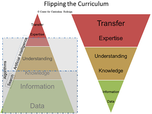
“What we need to test for is Transfer – the ability to use something we have learned in a completely different context. This has always been the goal of an Education, but now algorithms will allow us to focus on that goal even more, by ‘flipping the curriculum’.” — Charles Fadel
If Child A has memorized the data in her head while Child B has to look up the answers, some might argue that Child A is smarter than Child B. I would argue that AI has leveled the playing field for Child A and Child B, particularly if Child B is digitally literate, creative and passionate about learning. What are your thoughts?
First, let’s not conflate memory with intelligence, which games like Jeopardy implicitly do. The fact that Child A memorized data does not mean they are “smarter” than Child B, even though memory implies a modicum of intelligence. Second, even Child B will need some level of content knowledge to be creative, etc. Again, this is not developed in thin air, per the conversation above.
So it is a false dichotomy to talk about Knowledge or Competencies (Skills/Character/Meta-learning), it has to be Knowledge (modernized, curated) and Competencies. We’d want children to both Know and Do, with creativity and curiosity.
Lastly, we need to identify the Essential Content and Core Concepts for each discipline – that’s what the curation effort must achieve so as to leave time and space for deepening the disciplines’ understanding and developing competencies.
Given the impact of AI today and the advancements we expect each year, when should (all) school districts introduce open laptop examinations to allow students equal access to information and place emphasis on their thinkingskills?
The question has more to do with Search algorithms than with AI, but regardless, real-life is open-book, and so should exams be alike. And yes, this will force students to actually understand their materials, provided the tests do more than multiple-choice trivialities, which by the way we find even at college levels for the sake of ease of grading.
What we need to test for is Transfer – the ability to use something we have learned in a completely different context. This has always been the goal of an Education, but now algorithms (search, AI) will allow us to focus on that goal even more, by “flipping the curriculum”.
Today, if a learner wants to do a deep dive into any specific subject, AI search allows them to do this outside of classroom time. What do you say to a history teacher who argues there’s no need to revise subject content in his classroom?
For all disciplines, not just History, we must strike the careful balance between “just-in-time, in context” vs “just-in-case”. Context matters to anchor the learning: in other words, real-world projects give immediate relevance for the learning, which helps it to be absorbed. And yet projects can also be time-inefficient, so a healthy balance of didactic methods like lectures are still necessary. McKinsey has recently shown that today that ratio is about 25% projects, which should grow a bit more over time as education systems embed them better, with better teacher training.
Second, it should be perfectly fine for any student to do deep dives as they see fit, but again in balance: there are other competencies needed to becoming a more complete individual, and if one is ahead of the curve in a specific topic, it is of course very tempting to follow one’s passion. And at the same time, it is important to make sure that other competencies get developed too. So, balance and a discriminating mind matter.
Employers consider ethics, leadership, resilience, curiosity,mindfulness and courage as being of “very high” importance to preparing students for the workplace. How does your curriculum satisfy employers’ demands today and in the years ahead?
These Character qualities are essential for employers and life needs alike, and they have converged away from the false dichotomy of “employability or psycho-social needs.” A modern curriculum ensures that these qualities are developed deliberately, systematically, comprehensively, and demonstrably. This is achieved by matrixing them with the Knowledge dimension, meaning teaching Resilience via Mathematics, Mindfulness via History, etc. Employers have a mixed view and success as to how to assess these qualities, so it is a bit unfair that they would demand specificity they do not have. And it is also unfitting of school systems to lose relevance.
people, education, technology and exam concept – close up of students with smartphones taking picture of books page and making cheat sheet in school library
“Educators have been tone-deaf to the needs of employers and society to educate broad and deep individuals, not merely ones that may go to college. The anchoring of this problem comes from university entrance requirements.” — Charles Fadel
There is a significant gap between employers’ view of the preparation levels of students and the views of students and educators. The problem likely exists partly because of incorrect assumptions on both sides, but there are also valid deficiencies. What specific inadequacies are behind this gap? What system or process can be devised to resolve this issue?
On one side, employers are expecting too much and shirking their responsibility to bring up the level of their employees, expecting them to graduate 100% “ready to work” and having to spend nothing more than job-specific training at best. On the other side, educators have been tone-deaf to the needs of employers and society to educate broad and deep individuals, not merely ones that may go to college.
The anchoring of this problem comes from university entrance requirements (in the US, AP classes, etc.) and their associated assessments (SAT/ACT scores). They have for decades back-biased what is taught in schools, in a very self-serving manner – narrowly as a test of whether a student will succeed at university. It is time to deconstruct the requirements to broaden/deepen them to serve multiple stakeholders. For the Silo, C.M. Rubin.
(All photos are courtesy of our friends at CMRubinWorld)
C. M. Rubin and Charles Fadel
Join me and globally renowned thought leaders including Sir Michael Barber (UK), Dr. Michael Block (U.S.), Dr. Leon Botstein (U.S.), Professor Clay Christensen (U.S.), Dr. Linda Darling-Hammond (U.S.), Dr. MadhavChavan (India), Charles Fadel (U.S.), Professor Michael Fullan (Canada), Professor Howard Gardner (U.S.), Professor Andy Hargreaves (U.S.), Professor Yvonne Hellman (The Netherlands), Professor Kristin Helstad (Norway), Jean Hendrickson (U.S.), Professor Rose Hipkins (New Zealand), Professor Cornelia Hoogland (Canada), Honourable Jeff Johnson (Canada), Mme. Chantal Kaufmann (Belgium), Dr. EijaKauppinen (Finland), State Secretary TapioKosunen (Finland), Professor Dominique Lafontaine (Belgium), Professor Hugh Lauder (UK), Lord Ken Macdonald (UK), Professor Geoff Masters (Australia), Professor Barry McGaw (Australia), Shiv Nadar (India), Professor R. Natarajan (India), Dr. Pak Tee Ng (Singapore), Dr. Denise Pope (US), Sridhar Rajagopalan (India), Dr. Diane Ravitch (U.S.), Richard Wilson Riley (U.S.), Sir Ken Robinson (UK), Professor Pasi Sahlberg (Finland), Professor Manabu Sato (Japan), Andreas Schleicher (PISA, OECD), Dr. Anthony Seldon (UK), Dr. David Shaffer (U.S.), Dr. Kirsten Sivesind (Norway), Chancellor Stephen Spahn (U.S.), Yves Theze (LyceeFrancais U.S.), Professor Charles Ungerleider (Canada), Professor Tony Wagner (U.S.), Sir David Watson (UK), Professor Dylan Wiliam (UK), Dr. Mark Wormald (UK), Professor Theo Wubbels (The Netherlands), Professor Michael Young (UK), and Professor Minxuan Zhang (China) as they explore the big picture education questions that all nations face today.
C. M. Rubin is the author of two widely read online series for which she received a 2011 Upton Sinclair award, “The Global Search for Education” and “How Will We Read?” She is also the author of three bestselling books, including The Real Alice in Wonderland, is the publisher of CMRubinWorld and is a Disruptor Foundation Fellow.
The Metropolitan Museum of Art Launches New Immersive Virtual Reality and Online Feature with Iconic Works from Its Collection The Temple of Dendur and works from the Arts of Oceania galleries have been transformed for virtual reality (VR) experience and on the web
The Met’s new features, created in collaboration with the platform Atopia, introduce a new way for cultural institutions around the world to build their own VR and online exhibitions(New York, November, 2025)— The Metropolitan Museum of Art has launched two new virtual reality (VR) features, Dendur Decoded and Oceania: A New Horizon of Space and Time, that explore the Museum’s beloved Temple of Dendur and monumental works from the Oceanic art collection in the newly reopening Michael C. Rockefeller Wing—such as the Ceremonial House Ceiling from the Kwoma people of Papua New Guinea, the Asmat bisj poles, and Atingting kon(slit gongs) from Vanuatu—in 3D. The experiences will allow global audiences to view these treasured galleries and works using a personal VR headset or on The Met’s website. Designed in collaboration with Atopia, a platform for immersive art and culture, The Met’s virtual experiences introduce a new way for art institutions to create and publish their own VR and web features, providing more digital access to VR innovations across the museum field.
The Met’s first VR experiences, Dendur Decoded and Oceania: A New Horizon of Space and Time were developed in close consultation with Met curators. They feature original, innovative storytelling and high-resolution 3D scans created by The Met’s Imaging team. This experience allows virtual visitors to delve into artworks through movement, sound, interaction, and play. From stepping inside the Temple of Dendur to bringing the 17-foot bisj poles to eye level, these virtual experiences offer a singular opportunity to explore these iconic works.
“The Met collection is enjoyed by millions of visitors a year, and by exploring the vast possibilities of virtual spaces, we can offer unparalleled cultural experiences to audiences no matter where they are located,” said Max Hollein, The Met’s Marina Kellen French Director and CEO. “These two new VR and web features foreground compelling storytelling and curatorial scholarship, and they provide immersive, participatory access to some of The Met’s remarkable works of art.”
Annabell Vacano, founder of Atopia, said, “Until now, immersive exhibitions were bespoke and expensive. We created Atopia so museums of all sizes could design, publish, and scale interactive storytelling so their collections can be accessed from anywhere in the world. The Met has been an incredible partner in designing Atopia’s storytelling tools, and it’s been an honor to work with their world-class teams.”
Dendur Decoded The Dendur DecodedVR and web experience is organized as a vividly detailed adventure arranged in four “acts” and includes over 150 newly presented pieces of content, including materials (images and video) from archives at The Met and UNESCO. The content was created in collaboration with Isabel Stünkel, Curator, Department of Egyptian Art, and Erin Peters, Assistant Professor, Art History & Visual Culture at Appalachian State University; with support from Diana Craig Patch, Lila Acheson Wallace Curator in Charge of Egyptian Art, and Janice Kamrin, Curator in Egyptian Art at The Met.
It begins with “Act I: Explore Dendur,” which introduces the Temple and helps visitors learn how to read aspects of the temple’s decoration, and continues with “Act II: Dendur in Nubia,” presenting a 3D and 360-degree film about the Temple of Dendur’s original location along the West bank of the Nile River and how it was dismantled as part of the international UNESCO Campaign to Save the Monuments of Nubia to protect it from being submerged beneath Lake Nasser and then awarded to the United States in 1967. “Act III: Reconstructing Dendur” invites visitors to virtually rebuild part of the temple and learn how The Met reassembled it in New York in a new gallery that was opened to the public on September 27, 1978. “Act IV: Reflection” showcases past MetLiveArts performances and the ways in which contemporary artists have been inspired by the Temple. There is also an optional opportunity to leave a personal contemplation or observation through a voice note.
Oceania: A New Horizon of Space and Time Oceania: A New Horizon of Space and Time celebrates the dazzling Oceanic works in the Museum’s newly reopened Michael C. Rockefeller Wing. Fifteen objects are contextualized with sound, story, and a spatial design inspired by an outdoor environment that evokes the Pacific Islands. Within the space, these objects are accompanied by illuminating content such as immersive original audio and Pacific storytelling, archival imagery, 360-degree video, and high-resolution 3D models. Featuring works from across The Met collection of Oceanic art, highlights in the VR and web experience include The Met’s impressive Ceremonial House Ceiling, which evokes the polychrome interior of a men’s ceremonial house in the Sepik River region of Papua New Guinea five soaring upright spirit poles (bisj) from the Asmat people of Western New Guinea; and the 14-foot-tall Atingting kon (slit gong) from Vanuatu.
In this exploratory environment there is a lush virtual gallery populated by the 3D-scanned objects and immersive soundscapes. Examples include the Sawos Ancestor Figure, which invites close looking through a compelling audio story about a battle in which the ancestral figure came to life, paired with an interactive 3D model. The Ceremonial House Ceiling includes a game where visitors discover motifs across the 270 pangal (painted panels), including crocodiles, insects, and cassowaries. The Body Mask, created by an Asmat artist, includes contemporary photography by Joshua Irwandi, a documentary photographer based in Jakarta, Indonesia, showing how these masks are made and worn by the Asmat people of southwest New Guinea. For the Silo, Jarrod Barker.
Developed along with Maia Nuku, The Met’s Evelyn A. J. Hall and John A. Friede Curator for Arts of Oceania, and Sylvia Cockburn, Senior Research Associate for Arts of Oceania, the experience will be animated with voices from across the Pacific Islands, including a greeting by Michael Mel (PhD, performance artist, lecturer, curator, and teacher and currently Senior Lecturer and Head of Expressive Arts Department at the University of Goroka), and a concluding sunset ceremony by Che Wilson (Ngāti Rangi-Whanganui, Tūwharetoa, Mōkai Pātea, Ngāti Apa, Ngā Raurua), a Māori leader with a career that spans cultural advocacy, governance, and leadership.
VR and Online Innovations for the Cultural Sector For The Met’s virtual experiences, the Museum’s Emerging Technology and Digital department worked collaboratively with Atopia to develop a feature that will enable museums of all sizes to design and publish similar immersive exhibitions in-house. Through a “no-code” editor available on the platform, museum curators and designers can drag and drop images, 3D scans, and didactic information from their collections into virtual spaces. These can then be launched on the platform, becoming instantly available on the web and in VR.
Access and Availability The two immersive exhibitions are available now for free on The Met’s website and on Meta Quest 2/3/3s Audio across the experience is closed caption.
Atopia is compatible with both standard web browsers on a desktop and laptop and on personal VR headsets. It also supports both individual and invite-only multiplayer visits.
Related Programs These VR and web features will also be activated through several events, including Met Expert Talks. These talks include the opportunity for Museum visitors to interact with the virtual experiences on headsets provided by The Met for a deeper and more contextualized viewing. There will also be VR pop-ups at Teens Take The Met on May 15, 2026, as well as during an upcoming Teen Friday Career Labs, where teens can hear directly from the VR creative team. For homebound audiences unable to visit the new Arts of Oceania galleries in person, special Collection Tours will be offered for Oceania: A New Horizon of Space and Time via headsets provided by the Museum. More details and VR events at The Met will be announced.
Credits Dendur Decoded and Oceania: A New Horizon of Space and Time were created with a cross-disciplinary team from across The Met, led by Brett Renfer, Senior Project Manager of Emerging Technologies, along with Curatorial, Education, Imaging, and Digital.
This project is made possible by the Director’s Fund.
About The Metropolitan Museum of Art The Met presents art from around the world and across time for everyone to experience and enjoy. The Museum lives in two iconic sites in New York City—The Met Fifth Avenue and The Met Cloisters. Millions of people also take part in The Met experience online. Since it was founded in 1870, The Met has always aspired to be more than a treasury of rare and beautiful objects. Every day, art comes alive in the Museum’s galleries and through its exhibitions and events, revealing both new ideas and unexpected connections across time and across cultures. Discover more at metmuseum.org.
About Atopia Atopia is a new way to experience culture online. From any web browser or VR headset, audiences can step inside immersive exhibitions designed by leading museums worldwide. Our no-code platform empowers cultural institutions to create and share virtual experiences at scale—bringing exhibitions to global audiences beyond physical walls. Our mission: to open access to culture everywhere. Discover more at https://atopia.space
AWS Outage Created “Perfect Storm” for Social Engineering Attacks
Last week Amazon Web Services (AWS) went down worldwide, including here in Canada, causing a ripple effect, from governments and local municipalities, to enterprises, small businesses and the individuals who rely on these services daily.
AWS is a cloud-based service thousands of major companies use to not only store their data, but run their apps and software for many critical business services.
Whether basic communications using apps such as Snapchat, Signal and Reddit to airlines such as Delta and United reporting disruptions to their customer facing operations, when these services go down it highlights the reliance on just a few cloud services companies (AWS, Microsoft Azure, and Google Cloud) to ‘run the country’ so to speak.
The AWS outage has further impacted shopping websites, banking apps, and even streaming and smart homes devices.
And while organizations scramble to ensure business operations continue to run, it’s also an opportunity for individuals to do a quick check-in on their own cyber hygiene.
Cybercriminals and hackers can easily take advantage of these types of outages to deploy an array of social engineering attacks.
Whether in the office or at home, nothing is more frustrating than losing the ability to access files and documents, and communicate with business associates or loved ones, especially in an emergency or crisis.
Hackers who rely on mass urgency and panic will see this as an opportunity to take advantage of people’s heightened emotions with phishing emails offering to “fix” the issue and get you back online and into your accounts or apps.
But in reality, these scammers are looking to steal your personal information, such as login credentials by tricking you into updating your software or resetting your password.
During major outages, users should avoid clicking on any links in emails, texts and pop-ups claiming to be able to fix the outage.
Additionally, double check that any alerts or update messages from organizations, such as your bank or payment apps, are verified from the official website or app.
This is the time to make sure you are using a strong password and multifactor authentication to prevent any unauthorized access to your accounts.
Delay Things
However, individuals should also delay making sensitive transactions, such as major financial transactions, resetting your password, or installing critical software updates, until the service in question has been announced as officially restored.
Furthermore, when the service disruption has ended, users should also monitor any affected accounts for unusual activity, discrepancies, and duplicate or fraudulent transactions.
Finally, this is an excellent reminder for individuals to make sure they have a back-up system in place to access important documents and for communications.
This can be as easy as keeping a secondary email account or even a back-up mobile phone. For the Silo, Stefani Schappert.
ABOUT THE AUTHOR
Stefanie Schappert, MSCY, CC, Senior Journalist at Cybernews, is an accomplished writer with an M.S. in cybersecurity, immersed in the security world since 2019. She has a decade-plus experience in America’s #1 news market working for Fox News, Gannett, Blaze Media, Verizon Fios1, and NY1 News. With a strong focus on national security, data breaches, trending threats, hacker groups, global issues, and women in tech, she is also a commentator for live panels, podcasts, radio, and TV. Earned the ISC2 Certified in Cybersecurity (CC) certification as part of the initial CC pilot program, participated in numerous Capture-the-Flag (CTF) competitions, and took 3rd place in Temple University’s International Social Engineering Pen Testing Competition, sponsored by Google. Member of Women’s Society of Cyberjutsu (WSC), Upsilon Pi Epsilon (UPE) International Honor Society for Computing and Information Disciplines.
ABOUT CYBERNEWS
Friends of The Silo, Cybernews is a globally recognized independent media outlet where journalists and security experts debunk cyber by research, testing, and data. Founded in 2019 in response to rising concerns about online security, the site covers breaking news, conducts original investigations, and offers unique perspectives on the evolving digital security landscape. Through white-hat investigative techniques, Cybernews research team identifies and safely discloses cybersecurity threats and vulnerabilities, while the editorial team provides cybersecurity-related news, analysis, and opinions by industry insiders with complete independence.
Cybernews has earned worldwide attention for its high-impact research and discoveries, which have uncovered some of the internet’s most significant security exposures and data leaks. Notable ones include:
Cybernews researchers discovered multiple open datasets comprising 16 billion login credentials from infostealer malware, social media, developer portals, and corporate networks – highlighting the unprecedented risks of account takeovers, phishing, and business email compromise.
Cybernews researchers analyzed 156,080 randomly selected iOS apps – around 8% of the apps present on the App Store – and uncovered a massive oversight: 71% of them expose sensitive data.
Recently, Bob Dyachenko, a cybersecurity researcher and owner of SecurityDiscovery.com, and the Cybernews security research team discovered an unprotected Elasticsearch index, which contained a wide range of sensitive personal details related to the entire population of Georgia.
Audio-Technica expands turntable accessory offerings for all vinyl enthusiasts
Stow, OH, October, 2025 — Our friends at Audio-Technica, a leading innovator in transducer technology for over 60 years, are excited to launch a new range of turntable accessories designed to help vinyl listeners achieve the best from their record collections. The latest additions include two new slip-mats, precision alignment tools and a stainless-steel disc stabilizer. These new additions join Audio-Technica’s established lineup of turntable accessories including the AT6012 Record Cleaning Kit, stylus cleaners and more, expanding a complete family of products designed to help vinyl users care for and enjoy their collections to the fullest.
New to the Audio-Technica Slipmat series is the AT-SMCR2 Cork-Rubber Slipmat (MAP: $35.00 usd/ $49.00 cad) and AT-SMC1 Cork Slipmat (MAP: $25.00 usd/ $35.00 cad). The AT-SMCR2 is engineered from a premium blend of cork and rubber to absorb a wide range of vibrations, particularly at lower frequencies, delivering clearer audio reproduction. The cork-rubber blend also provides antistatic properties to reduce pops and clicks caused by static discharge. For listeners seeking a simpler option, the AT-SMC1 provides excellent resonance control and a stable playback surface without shedding particles or attracting dust like traditional felt mats.
Beyond vibration control, Audio-Technica introduces two new cartridge alignment tools designed to ensure precise playback geometry: the AT-VTAZ1 Azimuth + VTA Alignment Tool (MAP: $14.00 usd/ $20.00 cad) and AT-CAP1 Cartridge Alignment Protractor ($17.00 usd/ $24.00 cad). The AT-VTAZ1 allows users to achieve accurate tonearm height and cartridge azimuth adjustment. Proper alignment ensures even stylus wear, accurate channel balance, and minimal distortion. The AT-CAP1 utilizes the widely used Baerwald alignment method to set cartridge offset angle and null points to deliver optimal tracking and reduced distortion.
The new AT628a Stainless Steel Disc Stabilizer (MAP: $79.00 usd/ $111.00 cad )is designed to minimize resonance and keep records firmly in place during playback. The stabilizer accommodates even slightly warped records with two recessed inner rings on its underside for secure contact.
Rounding out the new launches are the AT-ST3 Speaker Stands (MAP: $59.00 usd/ $83.00 cad), designed to enhance the performance of the AT-SP3X or other similarly sized bookshelf speakers. Constructed from rigid alloy steel with vibration-damping cork feet, each stand provides stable support for speakers weighing up to 3 kg (6.6 lb). The 13-degree angled design directs sound upward for clearer projection and helps reduce sound wave reflections off hard surfaces, ensuring cleaner, more accurate audio reproduction.
For the Silo, Jarrod Barker.
Audio-Technica was founded in 1962 with the mission of producing high-quality audio for everyone. As we have grown to design critically acclaimed headphones, turntables and microphones, we have retained the belief that great audio should not be enjoyed only by the select few, but accessible to all. Building upon our analog heritage, we work to expand the limits of audio technology, pursuing an ever-changing purity of sound that creates connections and enriches lives.
ALUULA Composites, super-strong, lightweight polyethylene material is now being used to develop expandable habitats for NASA’s astronauts to live safely and comfortably on the moon for the 2027 planned landing.
This small company on Canada’s west coast is playing a big role to help astronauts return and orbit the moon in 2026.
Artemis II crew members (from left) CSA (Canadian Space Agency) astronaut Jeremy Hansen, and NASA astronauts Christina Koch, Victor Glover, and Reid Wiseman walk out of Astronaut Crew Quarters inside the Neil Armstrong Operations and Checkout Building to the Artemis crew transportation vehicles prior to traveling to Launch Pad 39B as part of an integrated ground systems test at Kennedy Space Center in Florida photo: NASA
ALUULA Composites recently signed an agreement with Max Space, an American company, to use its innovative composite material to build space habitats on the moon. The company’s ultra-high-molecular-weight polyethylene (UHMWPE) laminate will be used to create a large living and working area for NASA’s astronauts when they return to the moon in September 2026.
The innovative material was selected because it has eight times the strength-to-weight ratio of steel and is extremely durable, which is ideal for space travel.
The Max Space team with their new expandable space habitat. photo: Max Space
The first Max Space inflatable space habitat is slated to launch with SpaceX in 2026. The Max Space inflatables can be delivered into space in very small packages and then unfolded and expanded to create a much larger work space. For the Silo, Paul Clarke.
A recent consumer survey backed by similar results from Elon University reveals that AI adoption for car shopping is skyrocketing, rapidly becoming a standard part of the automobile buying process. This as fully one in four buyers have already used AI tools this year to research, compare prices, negotiate and otherwise outsmart dealerships, and an overwhelming 88% found it helpful. Signaling a seismic shift in the way North Americans are now shopping for cars, nearly half of consumers indicated plans to use AI in their next purchase. Not just for buyer benefits, dealerships are gleaning critical business intelligence from AI to inform sales strategies, train staff and elevate customer engagement. The below report from our friends at CarEdge, which offers its own AI Negotiator car buying tool saving shoppers thousands, details the first data-backed look at how AI tools are reshaping the car buying experience.
Mornine- AI powered car dealership robot.
Study: 1 in 4 Car Buyers Tap AI for Better Deals
Artificial intelligence is changing the way North Americans buy cars, and it’s a transition that is happening quickly. In the first-ever survey of its kind, CarEdge asked 500 car shoppers if they’re using AI tools like ChatGPT to research, compare, and negotiate during the car buying process. The results confirm a major shift is underway. One in four car buyers in 2025 are already using AI tools to gain an edge, and future buyers are even more likely to embrace these technologies.
Car buyers are finding AI to be a valuable tool. Among those who used tools like ChatGPT, Perplexity, Google Gemini, and others, 88% said it was helpful. AI is quickly becoming a trusted co-pilot for car buyers.
Key Findings: Car Buying Is Changing
The 2025 CarEdge AI & Car Buying Survey reveals a clear and growing trend: AI tools are quickly becoming part of the car buying process for a significant portion of consumers. Here are the standout findings:
1 in 4 Car Buyers Use AI
25% of car buyers in 2025 say they used or plan to use AI tools like ChatGPT during the shopping or buying process. This contrasts with a recent survey by Elon University that found 52% of Americans now use AI large language models. While signs point towards increased adoption of AI tools, the CarEdge survey found that most car buyers are still in the early stages of integrating these tools into high-stakes decisions like vehicle purchases. This suggests there’s still significant room for growth in AI adoption amongst car buyers.
AI Use Is Accelerating
Among those who haven’t bought a car yet this year, 40% say they are using or plan to use AI tools during their search or deal-making. This is nearly 3x higher than the 14% seen among those who already bought a car earlier in the year.
AI Tools Deliver Results
Among those who used AI:
88% say the tools were helpful
32% found them very helpful
60% used them “a lot” during the process
The AI Holdouts: Drivers Who Lease
Of the respondents who had already leased a car in 2025, none reported using any AI tools.
The AI-Adopting Buyer: Who’s Using It, and How?
AI adoption among car buyers is still in its early stages, but clear trends are beginning to emerge.
Among Buyers Who Already Purchased in 2025:
Just 14% of those who already bought a vehicle this year used AI tools during the process. Adoption rates were nearly identical across new and used buyers, with 14% in each group saying they used AI tools.
Among Future Car Buyers:
The numbers jump significantly when looking at those who haven’t yet bought in 2025. Among this group — who represent 39% of total respondents — 40% say they either already use or plan to use AI tools during their car search and buying process.
That’s more than triple the current usage rate among recent buyers, suggesting AI adoption is accelerating as awareness grows and tools become easier to use.
This group also appears to be more proactive: 60% of those who used AI tools during their buying journey said they used them “a lot,” while 40% used them only occasionally.
What Car Buyers Are Using AI Tools
AI tools are quickly becoming essential research companions for car shoppers looking to make more informed, confident decisions. After all, why go it alone when a wealth of automotive knowledge powered by large language models (LLMs) is right in your pocket?
Among buyers who used AI tools during their car purchase or lease process, here’s how they put them to work:
88% — Researching Vehicles
The most common use by far, AI tools helped buyers learn about different models, trims, features, and reliability. For many, it was like having an always-available expert to explain the pros and cons of their options.
64% — Comparing Prices and Market Values
Buyers used AI to better understand fair pricing, from invoice pricing to out-the-door.
44% — Learning Negotiation Strategies
Nearly half of AI users leaned on these tools to prepare for conversations with salespeople. Whether role-playing negotiation scenarios or asking how to spot add-on fees, this group used AI to level the playing field at the dealership.
11% — Exploring Finance and Lease Options
A much smaller portion of buyers used these tools to become familiar with leasing vs. financing, how to calculate payments, and similar queries.
Industry Implications
Car buying has always been tilted in favor of the dealership. Information asymmetry — what the dealer knows versus what the customer knows — has long been the source of consumer frustration, confusion, and overpayment.
That dynamic is beginning to shift.
This survey confirms what many in the industry are only starting to realize: AI is giving car buyers the upper hand. Tools like ChatGPT are helping consumers cut through the noise, ask smarter questions, and avoid common dealership traps. Instead of relying on guesswork or scattered advice, buyers are turning to AI for fast, personalized guidance at every step.
But one auto industry veteran has words of caution for buyers relying heavily on AI tools.
“It’s both surprising and a little scary to see how quickly people are turning to AI to guide such a major financial decision,” said Ray Shefska, Co-Founder of CarEdge. “While tools like ChatGPT can be powerful, they’re only as good as the data behind them. AI should complement your research, not replace your own critical thinking.“
That perspective underscores the real takeaway of this report: AI works best when it’s used thoughtfully as a tool, not as a crutch. In an age where automation raises fears of job loss or decision-making without human oversight, this survey offers a more optimistic view — one where technology helps everyday consumers make smarter choices. Used wisely, AI can help level the playing field and bring more transparency and fairness to the car buying experience.
Methodology
This survey was conducted by CarEdge between June 19 and June 24, 2025. A total of 500 U.S. respondents participated, recruited through the CarEdge email newsletter and social media channels. Questions were tailored based on buying status to better understand how and when AI tools were used in the car shopping process.
For the Silo, Karen Hayhurst.
About CarEdge Founded in 2019 by father-and-son team Ray and Zach Shefska, CarEdge is a leading platform dedicated to empowering car shoppers with free expert advice, in-depth market insights, and tools to navigate every step of the car-buying journey. From researching vehicles to negotiating deals, CarEdge helps consumers save money, time, and hassle, hundreds of thousands of happy consumers have used CarEdge to buy their car with confidence. With trusted resources like the CarEdge AI Negotiator tool, Research Center, Vehicle Rankings and Reviews, and hundreds of guides on YouTube, CarEdge is redefining transparency and fairness in the automotive industry. Follow them on YouTube, TikTok, X, Facebook, and Instagram for actionable car-buying tips and market insights. Learn more at www.CarEdge.com.
A horse and buggy. Excellent horse-power huh? People got tired of the nurturing it took to take care of a work horse. People wanted more and as with anything the need for something better fuels the spark for innovation. How about something to do work, but doesn’t need rest? Doesn’t need medication? Doesn’t need someone to shovel up its crap? Take this formula and you get the steam engine, not a crazy engine, but an engine none-the-less. Suddenly the glowing aura of potential is perceivable, right on the horizon. Now we can have multiple horse-power without the care. Still needed someone to shovel though.
The Horsey Horseless. Designed to prevent horses being frightened by a car.
Enter, the mother of current automotive technology today, the oil industry.
Instead of burning coal, why not find some ways to refine oil to be used as fuel sources to run things on? Who knows, we could have been running advanced versions of steam engines today? They actually can be made to be fairly efficient and clean using current technology and were quite practical cars back in 1918.
Then the internal combustion engine enters the scene the oil companies love this, and a mass marketed engine that is completely dependent on oil is born. Just think, this is awesome for business, these engines need oil for fuel and lubrication. Then all the different designs start flowing. (Off the top of my head and in no chronological order) The single cylinder, then 2, then 4, then 6, then the flathead V8. Now this is where we start to see major horse-power and design improvements. The trusty ole’ inline 6’s, the small block eating slant 6’s,The overhead valve V engine, big blocks, small blocks, Hemi’s. There are pancake engines, W engines, rotary engines, v-tecs, boxster engines and many, many more. (Not to mention all of the different fuel delivery systems!)
The cylinder and valves and crankshaft of the Internal Combustion Engine
The one thing that really makes me scratch my head is the fact that it took so long getting hybrids, smart-cars, electric cars, and hydrogen cars that are actually worth looking at and driving. I mean, why is it that I can take a full size 2008 Chevrolet Silverado with a 5.3 L vortec engine, put: a cold air intake, a magnaflow exhaust system, and a good edge products programmer, and I can get an average of over 36miles per gallon, with the same horse-power? Why is it that I (not being an automotive engineer) can do this, but you can’t just buy one with those numbers from the manufacturer?
Not to mention brown-gas converters that have been tested on most common engine types that can take, mineral water, and a reaction from current between two electrified plates (similar to a car battery) and create a safe amount of hydrogen gas as a by-product which can make your car run the same on half the amount of fuel. The thing that boggles me is that most people have never even heard of these. You can buy the plans off the internet (not as complicated as it sounds) or I can even get ready to install ones from my performance part supplier. I just find it strange that automotive technology and fuel sources have taken this long to start to veer just slightly away from oil (or as ‘ol Jed calls it “Texas tea”).
At one point we bridged the gap from a horse and buggy to a steam engine, and then to internal combustion. With the technology we have now, we should have much higher mpg’s and horse-power or an extremely viable alternative. It really makes me wonder where we might be now if this technology was steered in a different direction from the start. It’s been over 100 years now of improving the same technology using more or less the same fuel source. There are guys in the States who run their own garage refined deep fryer grease to power their small pickups and VW buses. There are guys who run pickups off wood-fire smoke. Just something to think about.
October, 2025 – Canada has world-class strength in AI research but continues to fall short in widespread adoption, according to a new report from the C.D. Howe Institute. On the heels of the federal government’s announcement of a new AI Strategy Task Force, the report highlights the urgent need to bridge the gap between research excellence and real-world adoption.
In “AI Is Not Rocket Science: Ideas for Achieving Liftoff in Canadian AI Adoption,” Kevin Leyton-Brown, Cinda Heeren, Joanna McGrenere, Raymond Ng, Margo Seltzer, Leonid Sigal, and Michiel van de Panne note that while Canada ranks second globally in top-tier AI researchers and first in the G7 for per capita publications, it is only 20th in AI adoption among OECD countries. “This matters for the economy as a whole, because such knowledge translation is a key vehicle for productivity growth,” the authors say. “It is terrible news, then, that Canada experienced almost no productivity growth in the last decade, compared with a rate 15 times higher in the United States.”
The authors argue that new approaches to knowledge translation are needed because AI is not “rocket science”: instead of focusing on a single industry sector, the discipline develops general-purpose technology that can be applied to almost anything. This makes it harder for Canadian firms to find the right expertise and for academics to sustain ties with industry. Existing approaches – funding academic research, directly subsidizing industry efforts through measures such as SR&ED and superclusters, and promoting partnerships through programs like Mitacs and NSERC Alliance – have not solved the problem.
Four ideas to help firms leverage Canadian academic strength to fuel their AI adoption include: a concierge service to match companies with experts, consulting tied to graduate student scholarships, “research trios” that link AI specialists with domain experts and industry, and a major expansion of AI training from basic literacy to dedicated degrees and continuing education. Drawing on their experiences at the University of British Columbia, the authors show how local initiatives are already bridging gaps between academia and industry – and argue these models should be scaled nationally.
“Canada’s unusual strength in AI research is an enormous asset, but it’s not going to translate into real-world productivity gains unless we find better ways to connect AI researchers and industrial players,” says Kevin Leyton-Brown, professor of computer science at the University of British Columbia and report co-author. “The challenge is not that AI is too complicated – it’s that it touches everything. That means new models of partnership, new incentives, and new approaches to education.”
AI Is Not Rocket Science- 4 Ideas in Detail
Idea 1: A Concierge Service for Matchmaking
We have seen that it is hard for industry partners to know who to contact when they want to learn more about AI. Conversely, it is at least as hard for AI experts to develop a broad enough understanding of the industry landscape to identify applications that would most benefit from their expertise. Given the potential gains to be had from increasing AI adoption across Canadian industry, nobody should be satisfied with the status quo.
We argue that this issue is best addressed by a “concierge service” that industry could contact when seeking AI expertise. While matchmaking would still be challenging for the service itself, it could meet this challenge by employing staff who are trained in eliciting the AI needs of industry partners, who understand enough about AI research to navigate the jargon, and who proactively keep track of the specific expertise of AI researchers across a given jurisdiction. This is specialized work that not everyone could perform! However, many qualified candidates do exist (e.g., PhDs in the mathematical sciences or engineering). Such staff could be funded in a variety of different ways: for example, by an AI institute; a virtual national institute focused on a given application area; a university-level centre like UBC’s Centre for Artificial Intelligence Decision-making and Action (CAIDA); a nonprofit like Mitacs; a provincial ministry for jobs and economic growth; or the new federal ministry of Artificial Intelligence and Digital Innovation.
Having set up an organization that facilitates matchmaking, it could make sense for the same office to provide additional services that speed AI adoption, but that are not core strengths of academics. Some examples include project management, programming, AI-specific skills training and recruitment, and so on. Overall, such an organization could be funded by some combination of direct government support, direct cost recovery, and an overhead model that reinvests revenue from successful projects into new initiatives.
Idea 2: Consultancy in Exchange for Student Scholarships
Many businesses that would benefit from adopting AI do not need custom research projects and do not want to wait a year or more to solve their problems. The lowest-hanging fruit for Canadian AI adoption is ensuring that industry is well informed about potentially useful, off-the-shelf AI technologies. We thus propose a mechanism under which AI experts would provide limited, free consulting to local industry. AI experts would opt in to being on a list of available consultants. A few hours of advice would be free to each company, which would then have the option of co-paying for a limited amount of additional consulting, after which it would pay full freight if both parties wanted to continue. The company would own any intellectual property arising from these conversations, which would thus focus on ideas in the public domain. If the company wanted to access university-owned IP, it could shift to a different arrangement, such as a research contract. This system would work best given a concierge service like the one we just described. The value offered per consulting hour clearly depends on the quality of the academic–industry match, and some kind of vetting system would be needed to ensure the eligibility of industry participants.
Why would an AI expert sign up to give advice to industry? All but the best-funded Canadian faculty working in AI report that obtaining enough funding to support their graduate students is a major stressor. Attempting to establish connections with industry is hard work, and such efforts pay off only if the industry partner signs on the dotted line and matching funds are approved. There is thus space to appeal to faculty with a model in which they “earn” student scholarships for a fixed amount of consulting work. For example, faculty could be offered a one- semester scholarship for every eight hours set aside for meetings with industry, meaning that one weekly “industry office hour” would indefinitely fund two graduate students. Consulting opportunities could also be offered directly to postdoctoral fellows or senior (e.g., post-candidacy) PhD students in exchange for fellowships. In such cases, trainees should be required to pass an interview, certifying that they have both the technical and soft skills necessary to succeed in the consulting role. The concierge service could help decide which industry partners could be routed to PhD students and which need the scarcer consulting slots staffed by faculty members.
The system would offer many benefits. From the industry perspective, it would make it straightforward to get just an hour or two of advice. This might often be enough to allow the company to start taking action towards AI adoption: there is a rich ecosystem of high-performance, reliable, and open-source AI tools; often, the hard part is knowing what tool to use in what way. Beyond the value of the advice itself, consulting meetings offer a strong basis for building relationships between academics and industry representatives, in which the academic plays the role of a useful problem solver rather than of a cold-calling salesperson. These relationships could thus help to incubate Mitacs/Alliance-style projects when research problems of mutual interest emerge (though also see our idea below about how restructuring such projects could help further).
For academics, the system would constitute a new avenue for student funding that would reward each hour spent with a predictable amount of student support. Furthermore, it would offer scaffolded opportunities to deepen connections with industry. The system would come with no reporting requirements beyond logging the time spent on consulting. The faculty member would be free to use earned scholarships to support any student (regardless, for example, of the overlap between the student’s research and the topics of interest to companies), increasing flexibility over the Mitacs/Alliance system, in which specific students work with industry partners. Students who self-funded via consulting would learn valuable skills and would expand their professional networks, improving prospects for post-graduation employment.
Finally, the system would also offer multiple benefits from the government’s perspective. It would generate unusually high levels of industrial impact per dollar spent (consider the number of contact hours between academia and industry achieved per dollar under the funding models mentioned in Section 3). All money would furthermore go towards student training. The system would automatically allocate money where it is most useful, directing student funding to faculty who are both eager to take on students and relevant to industry, all without the overhead of a peer-review process. And it would generate detailed impact reports as a side effect of its operations, since each hour of industry–academia contact would need to be logged to count towards student funding.
Idea 3: Grants for Research Trios
Our third proposal is an approach for expanding the Mitacs/Alliance model to make it work better for AI. Industry–academia partnerships leverage two key kinds of expertise from the academic side: methodological know-how for solving problems and knowledge about the application domain used for formulating such problems in the first place. In fields for which the set of industry partners is relatively small and relatively stable, it makes sense to ask the same academics to develop both kinds of expertise. In very general-purpose domains like AI, it holds back progress to ask AI experts to become domain experts, too. Instead, it makes sense to seek domain knowledge from other academics who already have it. We thus propose a mechanism that would fund “research trios” rather than bilateral research pairings. Each trio would contain an AI expert, an academic domain expert, and an industry partner. This approach capitalizes on the fact that there is a huge pool of academic talent outside core AI with deep disciplinary knowledge and a passion for applying AI. While such researchers are typically not in a position to deeply understand cutting-edge AI methodologies, they are ideally suited to serve as a bridge between researchers focused on AI methodologies and Canadian industrial players seeking to achieve real-world productivity gains. In our experience at UBC, the pool of non-AI domain experts with an interest in applying AI is considerably larger than the pool of AI experts. One advantage of this model is that projects can be initiated by the larger population of domain experts, who are also more likely to have appropriate connections to industry. Beyond this, involving domain experts increases the likelihood that a project will succeed and gives industry partners more reason to trust the process while a solution is being developed. The model meets a growing need for funding researchers outside computer science for projects that involve AI, rather than concentrating AI funding within a group of specialists. At the same time, it avoids the pitfall of encouraging bandwagon-jumping “applied AI” projects that lack adequate grounding in modern AI practices. Finally, it not only transfers AI knowledge to industry, but also does the same to both the domain expert and their students.
Idea 4: Greatly Expanded AI Training
As AI permeates the economy, Canada will face an increasing need for AI expertise. Today, that training comes mostly in the form of computer science degrees. Just as computer science split off from mathematics in the 1960s, AI is emerging today as a discipline distinct from computer science. In part, this shift is taking the form of recognizing that not every AI graduate needs to learn topics that computer science rightly considers part of its core, such as software engineering, operating systems, computer architecture, user interface design, computer graphics, and so on. Conversely, the shift sees new topics as core to the discipline. Most fundamental is machine learning. Dedicated training in AI will require a deeper focus on the mathematical foundations of probability and statistics, building to advanced topics such as deep learning, reinforcement learning, machine learning theory, and so on. Various AI modalities also deserve separate study, such as computer vision, natural language processing, multiagent systems, robotics, and reasoning. Training in ethics, optional in most computer science programs, will become essential.
Beyond dedicated training in the core discipline, we anticipate huge demand for broad-audience AI literacy training; for AI minors to complement other disciplinary specializations; for continuing education and “micro-credential” programs; and for executive education in AI. There is also a growing need for “AI Adoption Facilitators”: bridge-builders who can help established workers in medium-to-large organizations understand how data-driven tools could offer value in solving the problems they face. Training for this role would emphasize business principles and domain expertise, but would also require firmer foundations in machine learning and data science than are currently typical in those disciplines.
I graduated from the University of California at Berkeley about a decade ago with a degree in Mechanical Engineering. I received two job offers, one from SETI to work on high performance signal processing and the other from industry.
One does not simply walk away from SETI, so I had the pleasure of joining the Berkeley SETI Research Center (BSRC). I received a warm welcome and was promptly sent to West Virginia to help install a new SETI system at the Green Bank Telescope.
There was a steep learning curve, but I was fascinated by BSRC’s work and couldn’t wait to actually understand what was going on.
As it turns out, our group is looking to expand its computing power, providing the ability to look at more star systems with habitable planets, expand the involvement of volunteers and acquire larger volumes of data; in short, broaden the search and increase our chances of intercepting a signal. Now I’m working on setting up new servers, network hardware, and signal-processing systems at Green Bank. We’re hoping to get data flowing and recording soon, and make it available for the interested public.
From the 19th-century idea of drawing a giant Pythagorean triangle in the Siberian tundra to signal extraterrestrials, to our current collection of servers storing and analyzing data, it is not hard to see how much progress has already been made.
Running SETI software on your home computer looks like this.
Funding from the Breakthrough Initiatives is spawning new projects that would not have been otherwise possible. SETI@home is planning to work with Breakthrough Listen to collect and distribute data from the Green Bank and Parkes telescopes. However, in order to sustain the whole SETI@home effort we could still use support from our devoted SETI@home contributors.
Recently, I spent a day at the Bay Area Science Festival talking to kids and their adults. I was fascinated by just how stoked kids are about SETI. Some came with prepared questions and showed incredible curiosity and intelligence. The BSRC team is hoping to inspire kids to pursue science careers and I think searching for life beyond Earth is a great way to get them interested and involved. I hope you continue your support for this fascinating endeavor, and keep your eyes on the stars. For the Berkeley SETI Research Center team, Zuhra Abdurashidova.
Supplemental- via nemesis maturity YouTube channel
Wow Signal – Scientists say that if the signal came from extraterrestrials, they are likely to be an extremely advanced civilization, as the signal would have required a 2.2-gigawatt transmitter, vastly more powerful than any on Earth.
The signal bore the expected hallmarks of non-terrestrial and non-Solar System origin.
One summer night in 1977, Jerry Ehman, a volunteer for SETI, or the Search for Extraterrestrial Intelligence, may have become the first man ever to receive an intentional message from an alien world. Ehman was scanning radio waves from deep space, hoping to randomly come across a signal that bore the hallmarks of one that might be sent by intelligent aliens, when he saw his measurements spike.
The signal lasted for 72 seconds, the longest period of time it could possibly be measured by the array that Ehman was using. It was loud and appeared to have been transmitted from a place no human has gone before: in the constellation Sagittarius near a star called Tau Sagittarii, 122 light-years away.
All attempts to locate the signal again have failed, leading to much controversy and mystery about its origins and its meaning.
Considered by many to be The Holy Grail of Polyphonic Synthesis, this meticulously refurbished Oberheim FVS-1 took 88 hours of skilled vintage synth tech time via our friends at tonetweakers to perfect. The FVS-1 contains 4 classic Oberheim SEM modules, each providing a single dual oscillator voice. Sounds are dialed in manually on each module, with global control over the most tweaked parameters via the programmer module, where patches are also saved and recalled. Since each SEM is manually adjusted, it’s hard to get them sounding exactly the same. The result is a much more organic, slightly detuned, richer, truly magical sound than you’d get out of most other poly synths.
Famous users include Lyle Mays, 808 State, Depeche Mode, Styx, Pink Floyd, The Shamen, Gary Wright, Joe Zawinul and John Carpenter (yep the film director of The Thing, Big Trouble in Little China, Starman, Escape From New York and other classics often composed and recorded music for his movies). You won’t find a better example of this beautiful classic synthesizer, so if you’re looking for an exceptional 4 voice, now’s the time. Visit our friends at tonetweakers.com to learn more.
The OB Four Voice contains 4 SEMs and a mixer module. This beautiful instrument can play up to 8 oscillators at once, for insanely humongous sounds.
One of the first
The 4 voice was one of the first polyphonic synths. Each of the four Synthesizer Expander Modules ( SEM ) can be assigned to a different note. Splitting voices between modules is also possible, as is a monophonic unison mode. A single voice is surprisingly powerful, offering 2 oscillators, 2 envelopes (1 for filter, 1 for volume), an LFO, pulse width modulation and a real sweet multimode filter with sweep-able mode (which few synths offered). The programmer module allows fast saving and recall of programmed sounds. With a combined 8 oscillators, these sound unbelievably fat. Even a single SEM sounds great. In unison mode, play all VCOs on one key for one of the most powerful vintage synth sounds ever. Nothing sounds like it to us and we’ve played everything. This is a personal favorite. This FVS-1 has the standard configuration of modules: 4 x Synthesizer Expander Module ( SEM ) Keyboard Output module Polyphonic Keyboard module Programmer module.
No clangs or zaps
If you are an analog synth head who makes musical sounds, you need one of these. To avoid disappointment though, we would recommend anyone looking for a dedicated sound effects machine to go for something else. This 4 voice is fabulous at musical tones and can make some interesting sound effects but there are better choices for clangs, zaps, explosions and similar atonal timbres.
Other famous users include: Joe Zawinul, Chick Corea, Larry Fast (Synergy), Jan Hammer, Herbie Hancock, Human League, Michael McDonald / Doobie Brothers, Patrick Moraz, Steve Porcaro, The Shamen, Tim Simenon, Depeche Mode, Vince Clarke / Erasure, Tangerine Dream, Stevie Wonder and many other influential musicians who could afford one – this was a very expensive instrument when it came out!
Artificial Intelligence (AI) has infiltrated our lives for decades, but since the public launch of ChatGPT showcasing generative AI in 2022, society has faced unprecedented technological evolution.
With digital technology already a constant part of our lives, AI has the potential to alter the way we live, work, and play – but exponentially faster than conventional computers have. With AI comes staggering possibilities for both advancement and threat.
The AI industry creates unique and dangerous opportunities and challenges. AI can do amazing things humans can’t, but in many situations, referred to as the black box problem, experts cannot explain why particular decisions or sources of information are created. These outcomes can, sometimes, be inaccurate because of flawed data, bad decisions or infamous AI hallucinations. There is little regulation or guidance in software and effectively no regulations or guidelines in AI.
How do researchers find a way to build and deploy valuable, trusted AI when there are so many concerns about the technology’s reliability, accuracy and security?
That was the subject of a recent C.D. Howe Institute conference. In my keynote address, I commented that it all comes down to software. Software is already deeply intertwined in our lives, from health, banking, and communications to transportation and entertainment. Along with its benefits, there is huge potential for the disruption and tampering of societal structures: Power grids, airports, hospital systems, private data, trusted sources of information, and more.
Consumers might not incur great consequences if a shopping application goes awry, but our transportation, financial or medical transactions demand rock-solid technology.
The good news is that experts have the knowledge and expertise to build reliable, secure, high-quality software, as demonstrated across Class A medical devices, airplanes, surgical robots, and more. The bad news is this is rarely standard practice.
As a society, we have often tolerated compromised software for the sake of convenience. We trade privacy, security, and reliability for ease of use and corporate profitability. We have come to view software crashes, identity theft, cybersecurity breaches and the spread of misinformation as everyday occurrences. We are so used to these trade-offs with software that most users don’t even realize that reliable, secure solutions are possible.
With the expected potential of AI, creating trusted technology becomes ever more crucial. Allowing unverifiable AI in our frameworks is akin to building skyscrapers on silt. Security and functionality by design trump whack-a-mole retrofitting. Data must be accurate, protected, and used in the way it’s intended.
Striking a balance between security, quality, functionality, and profit is a complex dance. The BlackBerry phone, for example, set a standard for secure, trusted devices. Data was kept private, activities and information were secure, and operations were never hacked. Devices were used and trusted by prime ministers, CEOs and presidents worldwide. The security features it pioneered live on and are widely used in the devices that outcompeted Blackberry.
Innovators have the know-how and expertise to create quality products. But often the drive for profits takes precedence over painstaking design. In the AI universe, however, where issues of data privacy, inaccuracies, generation of harmful content and exposure of vulnerabilities have far-reaching effects, trust is easily lost.
So, how do we build and maintain trust? Educating end-users and leaders is an excellent place to start. They need to be informed enough to demand better, and corporations need to strike a balance between caution and innovation.
Companies can build trust through a strong adherence to safe software practices, education in AI evolution and adherence to evolving regulations. Governments and corporate leaders can keep abreast of how other organizations and countries are enacting policies that support technological evolution, institute accreditation, and financial incentives that support best practices. Across the globe, countries and regions are already developing strategies and laws to encourage responsible use of AI.
Recent years have seen the creation of codes of conduct and regulatory initiatives such as:
The Bletchley Declaration, Nov. 2023, an international agreement to cooperate on the development of safe AI, has been signed by 28 countries;
US President Biden’s 2023 executive order on the safe, secure and trustworthy development and use of AI; and
Governing AI for Humanity, UN Advisory Body Report, September 2024.
We have the expertise to build solid foundations for AI. It’s now up to leaders and corporations to ensure that much-needed practices, guidelines, policies and regulations are in place and followed. It is also up to end-users to demand quality and accountability.
Now is the time to take steps to mitigate AI’s potential perils so we can build the trust that is needed to harness AI’s extraordinary potential. For the Silo, Charles Eagan. Charles Eagan is the former CTO of Blackberry and a technical advisor to AIE Inc.
Living in space has significant effects on the human body. As we prepare for journeys to more distant destinations like Mars, humankind must tackle these risks to ensure safe travel for our astronauts.
With AI reshaping everything from finance to fast food, the $1.5T auto retail industry is finally facing its overdue disruption. The typical car-buying experience—riddled with hidden fees, lead bloat, pricing games and low trust—has remained stubbornly analog. But now, with 90% of dealerships in America (and growing % in Canada and Mexico) experimenting with AI tools and 1 in 4 buyers already using AI to shop, the tide is turning. Agentic AI technology is fundamentally reshaping one of the most significant purchases in a person’s life.
Zach Shefska, Co-Founder and CEO of CarEdge, asserts that agentic AI is the key to rebuilding trust, removing friction and leveling the playing field for both buyers and sellers. From AI-powered shopping assistants that negotiate on your behalf, to data tools that reveal deceptive dealership practices, Shefska is a pioneer in “agentic AI” — a new form of artificial intelligence bringing much-needed transparency to the industry.
The Broken Status Quo: Car buying is frustrating and inefficient for both consumers and dealerships—highlighting key stats like 72% sales staff turnover and 2% lead conversion from third-party platforms.
Lead Generation Platforms Are Failing: Legacy systems flood dealers with unqualified leads, drain resources, and deliver minimal value to consumers.
The Rise of Agentic AI in Auto Retail: Consumers are turning to tools like ChatGPT and CarEdge’s AI agent to navigate purchases with more confidence, speed, and clarity—25% are already doing it.
From Friction to Fluidity: Agentic AI replaces quantity with quality—streamlining the buyer’s journey, reducing information overload, and improving dealer efficiency.
The End of Pricing Games: AI tools now collect and publish out-the-door pricing from thousands of dealerships, exposing hidden fees and rewarding transparent sellers.
The Future of Negotiation: AI agents can negotiate on behalf of both buyers and sellers—minimizing stress, cutting transaction times from days to hours, and removing the adversarial edge.
Real-World Impact Stories: One buyer saved $1,280 and hours of back-and-forth using CarEdge’s agentic AI—illustrating AI’s practical value in real-life scenarios.
AI Helps Honest Dealers Win: In a trust-starved industry, AI gives reputable dealers a new way to stand out by offering full transparency and faster deals.
What’s Next for AI in Auto Retail: The emerging frontier: AI agents dynamically collecting and updating real-time pricing and inventory data across markets to offer true market intelligence.
For the Silo, Zach Shefska. Zach is CEO of CarEdge, a leading platform—founded by father-and-son team Ray and Zach Shefska—dedicated to empowering car shoppers with free expert advice, in-depth market insights and tools to navigate every step of the car-buying journey. From researching vehicles to negotiating deals, CarEdge helps consumers save money, time and hassle. Alsop with trusted resources like the CarEdge Research Center, Vehicle Rankings and Reviews, and hundreds of guides on YouTube, CarEdge is redefining transparency and fairness in the automotive industry. Connect with Shefska at www.CarEdge.com or on social media on YouTube, TikTok, X, Facebook, and Instagram.
Buckminster was a genius and his geodesic dome buildings were not only revolutionary in their construction but were also incredibly unique and memorable. Perhaps your grandparents attended Expo67 in Montreal (you guessed it, waaay back in 1967) and visited the United States Pavilion- read this snippet for a time capsule account:
“The United States exhibit, entitled Creative America, is designed to illustrate technological and esthetic inventiveness in the U.S.A.A huge transparent geodesic “bubble” contains a multi-level system of exhibit platforms interconnected by escalators, and walkways. The platforms support a variety of exhibit components specially selected or designed for the new environment created by the structure. Situated on Ile Sainte-Hélène close to the Métro station from which there is Minirail connection with the Expo-Express, the bubble is 20 stories high and has a spherical diameter of 250 feet .By day, the bubble glistens as the sun highlights the structure and, by night, the bubble “glows” from interior lighting. The interior exhibits reflect different aspects of the United States and include folk art, cinema and fine arts displays, as well as a space exhibit which is reached by a 125 foot escalator and a simulated lunar landscape supporting full scale lunar vehicles. A 300-seat theatre features a 3-screen color film showing the games children play.”
Photo- National Archives of Canada
If you think that was pretty amazing check out some of Buckminster’s buildings that unfortunately didn’t make it past the planning stage.
VENTURI SPACE PRESENTS MONA LUNA, THE EUROPEAN LUNAR ROVERMONA LUNA, designed by Sacha Lakic
Paris Air Show, Le Bourget, June 2025 – Venturi Space unveils MONA LUNA, its 100% European-built lunar rover. Designed to support the ambitions of the European Space Agency and the French CNES, the vehicle will be built at Venturi Space France’s facility in Toulouse. The ultimate aim is to provide Europe with a lunar-capable rover by 2030.
European autonomy in lunar mobility is a major strategic challenge. Venturi Space is helping to make that a reality with MONA LUNA, its upcoming lunar rover designed to meet the needs of ESA and national European space agencies. The vehicle will further Europe’s efforts to achieve technological independence in the field of lunar mobility, enabling it to get ahead of the industrial curve and achieve its space ambitions.
A project led by Venturi Space France Venturi Space France will oversee MONA LUNA’s development and space qualification from its base in Toulouse, coordinating every aspect of the process: onboard electronics, avionics, space-to-ground links, energy management systems, assembly, final integration, and acceptance testing in readiness for space flight. All with one clear objective: to deploy MONA LUNA at the Moon’s South Pole by 2030.
Backed by the ESA and CNES The European Space Agency is supporting Venturi Space’s efforts to design and develop the critical technologies required for a large lunar rover, capable of surviving multiple lunar nights. ESA’s support validates Venturi Space’s approach and highlights its expertise. The project will draw on the experience acquired from the programmes to develop the FLIP and FLEX rovers under a strategic partnership with US-based company Venturi Astrolab, Inc. Venturi Space is currently designing and building the hyper-deformable wheels that will be fitted to those vehicles, along with the associated electrical systems (in Switzerland) and high-performance batteries (in Monaco).
Using technology made in Europe MONA LUNA is designed to be carried into space by the Ariane 6.4 launch system and landed on the Moon’s surface by the European Argonaut lunar lander, while the rover itself will be equipped with a robotic arm to handle scientific instruments and payloads. It will be: – electrically powered, recharging via solar panels, – designed to move autonomously, – equipped with three high-performance batteries, – capable of carrying a wide range of payloads, – designed to survive multiple lunar nights, – capable of a top speed of 20 km/h, – designed to weigh a total of 750 kg.
The rover could also be used in an emergency to carry an astronaut in difficulty, as envisaged by the ESA and CNES in their feasibility studies. A clear commercial purpose MONA LUNA’s maiden mission will focus on purely scientific applications, but future deployments could be organized to meet demand from the European private sector for a variety of purposes, including carrying payloads to the South Pole, exploiting lunar resources (such as helium-3) in situ, or even public outreach campaigns. This approach will help establish a sustainable long-term economic model for the rover, in much the same way as the early development of terrestrial mobility.
Gildo Pastor, President of Venturi Space: “I’m still an explorer, first and foremost. Space is a new frontier, and MONA LUNA is how we are actually going to broach it. Alongside Europe, we aim to build an autonomous lunar exploration capability to meet the scientific, economic, and strategic challenges of tomorrow.”
Dr. Antonio Delfino, Director of Space Affairs at Venturi Space: “Our primary focus is to make ourselves fully available to the ESA and European national space agencies. With MONA LUNA, we aim to deliver major technological breakthroughs that will pave the way for extended lunar mobility.”
Summer, and thus driving season, is currently in full swing for much of Canada. Most of us that have them are trying to drive our classics every chance we get. Here are some vital reminders to heed if your vintage ride gets called up into everyday action.
Where I live is currently in the beautiful pocket of time where the mornings are cool yet bright and the sun only really gets hot in the middle of the afternoon. All of my cars love this weather, and I love driving just that little bit more. So I’m trying to drive as much as I can, and if you are doing the same, here are a handful of reminders for the times your vintage ride gets called up into more routine service.
Before we dive in though, it’s worth mentioning that old cars were once new cars. Someone drove and treated my Chevrolet Corvair the way I currently behave while behind the wheel of my wife’s Jeep Renegade—a daily driver. Traffic 30, 40, or even 90 years ago was radically different than traffic today, and many of our common-sense habits have shifted meaning to the point that what makes total sense for you in your old car will look insane to a common road user. While old cars require an additional amount of care and attention to be used regularly, driving your car is the best thing you can do for it. Don’t be scared of using the car exactly how it was intended.
Old cars have old brakes
Fresh wheel bearings and drums made for a big improvement in drivability and safety on my Model A Ford.Kyle Smith
It’s easy to get lured into driving like those around you, but be careful. Without notice, you’ll find yourself tailgating at the same distance as the modern cars, and when that line of cars taps the brakes, suddenly the concept of 5-mph bumpers doesn’t seem so comical.
Vintage brakes can be made to work very well with a bit of care and attention, but even I have to admit vintage designs and materials just cannot compare to modern brakes—that is before even mentioning driver assist systems like anti-lock braking or emergency braking. Give yourself plenty of room.
Check your fluids often
Kyle Smith
Modern cars have spoiled us with the ability to drive thousands of miles without opening the hood. Regardless of how you feel about the separation between driver and mechanic over time, driving your vintage car on more than just a couple weekends a month requires staying on top of topping of fluids.
Old engines can and often do consume oil at a rate much higher than modern engines. Add in even just a small leak and suddenly the bottom of the dipstick is bone dry and before long, so is the oil pickup. Engine oil also helps cool an engine, so keeping oil topped up helps for multiple reasons beyond just proper lubrication. Also keep an eye on brake fluid and coolant.
Modern car gauges are “normalized,” meaning that they often will be basically stationary while driving despite slight fluctuation in the pressures, temperatures, and levels they monitor. On older cars, a coolant temp gauge might rise slightly when caught at a long stoplight, but it might not actually be a cause for concern. Most automotive engines operate best when coolant temps are between 180 and 210 degrees Fahrenheit. Modern gauges will be stationary for that entire range, but an old-school mechanical gauge will transmit everything. This means coolant temp could drop slightly when you turn on the heater, or increase some with long periods of idling or while an air conditioner is cycling.
Make your escape plans
Smiley N. Pool/Houston Chronicle/Getty Images
Even in great condition, aging cars can and do break down. Think through what common failures might occur with your car and formulate a plan for how you will handle the situation. This can mean packing a tool kit, re-upping your roadside assistance membership, or choosing routes and times of day that will help ensure you have a smooth trip. Some vintage cars will have zero trouble in modern traffic, but if yours tends to overheat or get cranky sitting still, make sure that you scout an escape route, should you get snarled in traffic. Being stuck on the side of the road is infinitely better than being stuck in the middle of the road. Trust me. There are a few roads around town that I avoid in my vintage cars due to the lack of shoulder or safe place to veer off. Paranoid? Maybe a little, but I don’t want to get hit while sitting on the side of the road.
Be aware of your tires
Andrew Ganz
Modern tires are downright amazing and often go underappreciated. Since vintage cars get less mileage than their modern counterparts, a lot more people are willing to drive on older or poor-condition tires, sometimes out of pure ignorance or from lack of inspection. Tread depth and age are big considerations, but if you’re running modern reproductions of older tire designs, there is also the way those tires handle water. Siping and water control have a huge impact on handling and braking. You might have brand-new tires, but if the design is 50 years old, they are going to handle that way. Again, not a bad thing, but something to adjust to. For the Silo, Kyle Smith.
Why are so many people still struggling with brain fog, chronic fatigue, low energy, impaired memory, diminished focus, high stress and ADHD symptoms—even despite years of trying treatments for many? Neurotologist Dr. Kendal Stewart believes it’s because we’re too often treating symptoms, not causes. He’s spent the last 25 years addressing that with science-backed ways to help people at every age improve how they feel and function, both immediately and long-term. As an authority in everyday brain health, Dr. Kendal Stewart helps individuals optimize focus, memory, resilience and other brain health concerns by transforming complex neurological science into simple, actionable lifestyle-based strategies.
Dr. Stewart has spoken at length and has written many editorials to discuss real-world habits, tactics and solutions to reduce brain fog, feel more energized, support focus, maintain emotional balance, and preserve cognitive health as one ages. A variety of related topics that include:
What brain fog, anxiety, and immune dysfunction have in common—and how to address all three holistically
Fueling your brain and immune system based on your unique DNA
Actionable daily habits to support brain and immune system health
How your genetics dictate your brain & immune health–and how to decode it
Why the future of medicine is personalized and already here
What are neuroimmune disorders, and why are we seeing a rise in conditions like chronic pain?
How genetic testing removes guesswork in treating complex neurological conditions
Hope for the undiagnosed: Dr. Stewart’s approach to finding the ‘source’ when other treatments fail
Why we’re still getting brain fog wrong—and what to do instead
A neurotologist’s take on impaired memory, focus, stress and fatigue: stop treating just the symptoms
Easy ways to support your brain & immune system every day
Does your DNA hold the key to focus, energy & emotional balance?
Genetics meets neuroscience for personalized brain health
What distinguishes Dr. Stewart?
Medical Maverick: One of the few specialists bridging neurotology (brain-ear balance) and neuroimmune genetics to treat complex disorders.
DNA-Driven Results: Nearly every patient receives genetic testing to eliminate guesswork—a game-changer for conditions like autism, chronic fatigue, and concussions.
Science Meets Storytelling: From IV therapies to nutrigenomics, he translates cutting-edge science into actionable steps for families and high performers.
Media-Ready: A charismatic speaker and podcast personality with patented tech, a supplement line (Neurobiologix), and a mission to “recover” patients, not just manage symptoms.
About the Expert Dr. Stewart is a board-certified neurotologist and nationally recognized expert in neuroimmune disorders—including genetic abnormalities, chronic pain, ADD/ADHD and autism spectrum conditions. With advanced training in both surgery and cellular science, he’s made it his life’s work to uncover root causes and tailor individualized solutions through genetic testing, functional medicine, and integrative care. His approach emphasizes prevention as much as treatment, using lifestyle, nutrition, and nervous system support as daily fuel for better brain function. Through his work, he provides practical tools to regulate stress, stabilize energy and boost mental clarity.
He’s also a sought-after keynote speaker, inventor, and founder of multiple healthcare innovations, including GX Sciences, SensoryView, and Neurobiologix—a company dedicated to improving individual well-being by developing cutting-edge nutritional supplements rooted in the science of nutrigenomics. Dr. Stewart brings not only clinical authority but also an empowering, real-world lens—helping families, patients, and professionals better understand and improve nervous system and immune function. For the Silo, Karen Hayhurst.


 It’s hard to say exactly what the future holds, though Steve Jobs was seemingly pretty good at predicting it. In 1972 I had the unusual opportunity to be in a computer class with Steve Jobs. Of course, at the time he was just a nerdy teen and I was four years his junior. He and I would vie to play Tic-tac-toe on a 500 pound “computer” that our High School had recently purchased. Steve was obsessed with this machine. One day I asked Steve why he was so fixated on this refrigerator sized computer. He turned to me and said in an intense manner, “Don’t you see? This machine is going to change everything! It’s going to change the world!”


 MONA LUNA at Luna · Design: Sacha Lakic ©Venturi Space/Romero